Drawing with epicycles and the Fourier transform
In ancient times, the astronomer Ptolemy modeled the motion of celestial objects as uniform circular motion.
Of course, as seen from the Earth, the planets do not move in uniform circular motion, but the ancients believed for religious reasons that all celestial bodies had to. They therefore then began to adapt the model. Instead of moving about the Earth, a planet was held to move about a point called the deponent in a uniform circle called the epicycle, while the deponent moved about the Earth in uniform circular motion whose circle had a different radius and moved at a different rate.
As observations became more accurate, astronomers were forced to add more epicycles to fit the observed data. They had confidence in their model, because any new observation always fit the model as long as more epicycles were present.
Their confidence was misplaced; Kepler and Newton came up with much simpler models that explained the data. Moreover, using the Fourier transformation, one can model any piecewise-continuous path to arbitrary accuracy by adding enough epicycles.
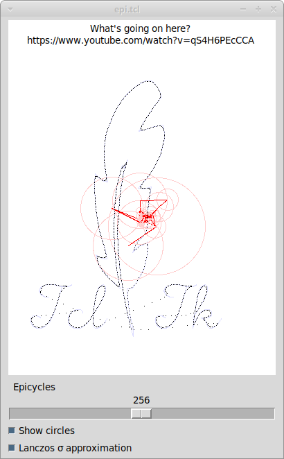
Herewith, KBK presents code to compute and display the orbit of the Tcl feather.
A sketch of what's happening:
- The path is defined as a sequence of {x y} pairs.
- The points on the path are resampled so that the resulting point list are approximately equally spaced, and there is a power-of-2 number of them.
- The resampled {x y} pairs are treated as complex numbers. They are passed to a Fast Fourier Transformation - which hands back the parameters of the epicycles. (This is the key step. For a gentle introduction to the mathematics, there is a three-part video series on the Fourier transform, including further epicycle drawing, culminating at 3Blue1Brown's channel on YouTube - and the links in the description go to further good introductory material.
- The resulting set of epicycles is usable as is, but because of a behaviour called the Gibbs phenomenon , there are large oscillations near the discontinuous jumps. The oscillations can be damped out by applying a low-pass filter - that is, making the fast-moving epicycles smaller. One popular filter to use is the Lanczos σ approximation. This particular filter almost eliminates the overshoot and ripples, at the cost of a slower jump and more spurious points in the gaps.
- The display logic is fairly straightforward use of the Tk canvas.
Jeff Smith 2019-07-21 : Below is an online demo using CloudTk. (The iFrame will go black for a while just wait for the demo to load.)
Please Note : This demo has a run time of 2 minutes.
# epi.tcl -- Demonstrate drawing with epicycles.
#
# What's going on here?  https://www.youtube.com/watch?v=qS4H6PEcCCA


package require Tk
package require math::constants
package require math::fourier

math::constants::constants pi
math::constants::constants eps

namespace path {tcl::mathop tcl::mathfunc}

# Linestrings to display using epicycles

set displayList {

    {
        60.0 399.5 54.0 399.5 48.0 396.5 45.0 390.5 48.0 384.5 57.0 381.5
        66.0 381.5 78.0 384.5 87.0 384.5 93.0 381.5
    }
    {
        78.0 384.5 72.0 405.5 66.0 423.5 60.0 435.5 54.0 441.5 48.0 444.5
        42.0 444.5 36.0 441.5 33.0 435.5 33.0 429.5 36.0 426.5 42.0 426.5
        48.0 429.5
    }
    {
        108.0 423.5 108.0 420.5 105.0 417.5 99.0 417.5 93.0 420.5 90.0 423.5
        87.0 429.5 87.0 435.5 90.0 441.5 96.0 444.5 105.0 444.5 114.0 438.5
        120.0 429.5
    }
    {
        120.0 429.5 126.0 420.5 135.0 405.5 138.0 399.5 141.0 390.5 141.0 384.5
        138.0 381.5 132.0 384.5 129.0 390.5 126.0 402.5 123.0 423.5 123.0 441.5
        126.0 444.5 129.0 444.5 135.0 441.5 138.0 438.5 144.0 429.5
    }

    {
        240.0 399.5 234.0 399.5 228.0 396.5 225.0 390.5 228.0 384.5 237.0 381.5
        246.0 381.5 258.0 384.5 267.0 384.5 273.0 381.5
    }
    {
        258.0 384.5 252.0 405.5 246.0 423.5 240.0 435.5 234.0 441.5 228.0 444.5
        222.0 444.5 216.0 441.5 213.0 435.5 213.0 429.5 216.0 426.5 222.0 426.5
        228.0 429.5
    }
    {
        267.0 429.5 273.0 420.5 282.0 405.5 285.0 399.5 288.0 390.5 288.0 384.5
        285.0 381.5 279.0 384.5 276.0 390.5 273.0 402.5 270.0 420.5 267.0 444.5
    }
    {
        267.0 444.5 270.0 435.5 273.0 429.5 279.0 420.5 285.0 417.5 291.0 417.5
        294.0 420.5 294.0 426.5 288.0 429.5 279.0 429.5
    }
    {
        279.0 429.5 285.0 432.5 288.0 441.5 291.0 444.5 294.0 444.5 300.0 441.5
        303.0 438.5 309.0 429.5
    }
    {
        181 457 172 422 166 390 162 363 159 332 158 302 160 275 162 250
        167 220 173 202 167 214 165 210 157 240 154 270 153 300 154 330
        157 360 162 388 145 372 132 356 127 339 135 344 143 345 141 334
        132 304 127 275 125 246 125 235 126 222 133 230 136 232 144 234
        141 220 139 203 139 183 142 163 154 133 164 117 172 107 186 95
        198 88 207 88 212 92 218 101 222 111 211 125 197 146 189 161
        200 158 211 154 224 152 226 164 226 172 220 196 210 215 202 227
        188 243 197 244 207 241 204 257 202 276 201 283 202 295 201 301
        198 309 189 319 186 321 180 336 188 327 196 325 202 320 201 340
        197 358 192 368 184 381 179 388 172 388 174 412 176 425 181 447
        181 457
    }
}

# Fill in points for a single segment
#    plistVar - Variable in caller containing the list  of points
#               under construction
#    dl - Arc length corresponding to the point spacing in plist
#    x0 y0 - Starting point of the segment
#    x1 y1 - Ending point of the segment
#    l0 - Arc length consumed up to this point
# Returns arc length accumulated to end of segment
# Appends discretization of the segment to the point list.

proc paintOneSegment {plistVar dl x0 y0 x1 y1 l0} {

    upvar 1 $plistVar plist

    set len [expr {hypot($x1-$x0, $y1-$y0)}]
    set l1 [expr {$l0 + $len}]

    while {1} {
    set t [llength $plist]
    set l [expr {$dl * $t}]
    if {$l > $l1} break
    set x [expr {($x0*($l1 - $l) + $x1*($l - $l0))/($l1 - $l0)}]
    set y [expr {($y0*($l1 - $l) + $y1*($l - $l0))/($l1 - $l0)}]
    lappend plist [list $x $y]
    }

    return $l1
}

# Paints one linestring into the point list
#    plistVar - Variable in caller's scope containing the point list
#    dl - Arc length corresponding to the point spacing in plist
#    lstr - List of {x y} pairs making up the linestring
#    l - Arc length accumulated so far
# Returns arc length accumulated to end of linestring
# Appends discretization of the linestring to the point list.

proc paintOneLinestring {plistVar dl lstr l} {

    upvar 1 $plistVar plist

    foreach {x y} $lstr {
    if {[info exists lastx]} {
        set l [paintOneSegment plist $dl $lastx $lasty $x $y $l]
    }
    set lastx $x
    set lasty $y
    }

    return $l
}

# Calculates arc length for a single linestring
#    lstr - Linestring to calculate
# Returns the arc length

proc linestringArcLength {lstr} {

    set l 0.0

    foreach {x y} $lstr {
    if {[info exists lastx]} {
        set l [expr {$l + hypot($x-$lastx, $y-$lasty)}]
    }
    set lastx $x
    set lasty $y
    }

    return $l
}

# Calculates total arc length for the drawing
#    lstrs - List of linestrings
# Returns the arc length

proc totalArcLength {lstrs} {

    set l 0.0
    foreach lstr $lstrs {
    set l [expr {$l + [linestringArcLength $lstr]}]
    }

    return $l
}

# Paints the whole drawing into the point list
#    lstrs - List of linestrings to paint
# Returns the point list produced

proc paintDrawing {lstrs} {

    set ltotal [totalArcLength $lstrs]
    set n [expr {1 << int(log($ltotal)/log(2.) + 1)}]
    set dl [expr {$ltotal / $n}]

    set plist {}
    set l 0.0

    foreach lstr $lstrs {
    set l [paintOneLinestring plist $dl $lstr $l]
    }

    return $plist
}

# Draw the epicycles at a single time point. c is the canvas to draw in.
# F is the Fourier coefficients. th is the current phase angle (0 .. 2pi)
# and n is number of epicycle pairs to consider.

proc drawEpicycles {c F th n} {

    variable lanczosSigma
    variable showCircles

    $c delete withtag epicycle
    $c delete withtag spoke

    set x 0.0
    set y 0.0

    for {set i 0} {$i <= $n} {incr i} {

        set ntheta [expr {$i * $th}]
        set cs [expr {cos($ntheta)}]
        set sn [expr {sin($ntheta)}]

        lassign [lindex $F $i] xi yi

        # Lanczos sigma approximation, to quiet the Gibbs phenomenon

        if {$lanczosSigma} {
            set sigma [expr {sinc($::pi * $i / $n)}];
            set xi [expr {$sigma * $xi}]
            set yi [expr {$sigma * $yi}]
        }

        set xx [expr {$x + $xi * $cs - $yi * $sn}]
        set yy [expr {$y + $yi * $cs + $xi * $sn}]
        if {$i > 0} {
            if {$showCircles} {
                set m [expr {hypot($xi, $yi)}]
                $c create oval [- $x $m] [- $y $m] [+ $x $m] [+ $y $m] \
                    -width 1 -fill {} -outline #ffcccc -tags epicycle
            }
            $c create line $x $y $xx $yy -width 0 -fill red -tags spoke
        }
        set x $xx
        set y $yy

        if {$i == 0} continue

        set i2 [expr {[llength $F] - $i}]
        lassign [lindex $F $i2] xi yi
        if {$lanczosSigma} {
            set xi [expr {$sigma * $xi}]
            set yi [expr {$sigma * $yi}]
        }
        set sn [expr {-$sn}]

        set xx [expr {$x + $xi * $cs - $yi * $sn}]
        set yy [expr {$y + $yi * $cs + $xi * $sn}]
        if {$i > 0} {
            if {$showCircles} {
                set m [expr {hypot($xi, $yi)}]
                $c create oval [- $x $m] [- $y $m] [+ $x $m] [+ $y $m] \
                    -width 1 -fill {} -outline #ffcccc -tags epicycle
            }
            $c create line $x $y $xx $yy -width 0 -fill red -tags epicycle
        }
        set x $xx
        set y $yy

    }
    .c create line $x $y [+ $x 1] $y -fill black -tags trail

    return
}

# This is a bad way to compute sinc, but good enough for our purposes

proc tcl::mathfunc::sinc {x} {
    if {abs($x) < $::eps} {
        return 1.0
    } else {
        return [expr {sin($x) / $x}]
    }
}

# Animates the display
#    when - milliseconds at which animate was last scheduled to wake up.

proc animate {when} {

    variable nstep
    variable F
    variable ncycles

    set then [expr {$when + 33}]

    drawEpicycles .c $F [expr {1.618034 * [incr nstep] * $::pi / 400}] \
        $ncycles
    .c raise spoke
    .c raise trail

    after [expr {$then - [clock milliseconds]}] [list animate $then]
}


# Updates number of pairs of epicycles
#    n - number of PAIRS of epicycles

proc updateCycles {n} {
    variable ncycles
    .c delete withtag trail
    set ncycles [expr {int($n / 2)}]
}


set showCircles 1
set lanczosSigma 1

# Make the GUI

grid [canvas .c -width 384 -height 512 -background white] \
     -padx 10 -pady {4 2} -sticky nsew
.c create text 192 5 -text "What's going on here?\nhttps://www.youtube.com/watch?v=qS4H6PEcCCA" -justify center -anchor n
grid [scale .s -command updateCycles -from 2 -to 512 -label Epicycles \
          -orient horizontal -length 384 -resolution 2 -showvalue 1] \
    -padx 10 -pady {2 2} -sticky ew
grid [ttk::checkbutton .ck -text "Show circles" -variable showCircles] \
    -sticky w -padx 10 -pady {2 2}
grid [ttk::checkbutton .ck2 -text "Lanczos \u03c3 approximation" \
          -variable lanczosSigma \
          -command {.c delete withtag trail}] \
    -sticky w -padx 10 -pady {2 4}

# bind .c <ButtonRelease-1> exit

# Make the point list to Fourier-transform

set plist [paintDrawing $displayList]

# Show the display list faintly

foreach fig $displayList {
    .c create line {*}$fig -width 0 -fill #ddddff
}

# FFT the point list, and rescale.

set F [math::fourier::dft $plist]
set F [lmap pair $F {
    lassign $pair i q
    lmap coord $pair {
        expr {$coord / [llength $plist]}
    }
}]

set nstep -1
set ncycles 128
.s set 256


animate [clock milliseconds]
Category Mathematics Category Graphics
arjen - 2019-07-22 06:40:31
Wonderful, both the live demo and the epicycles as such :). I just wonder how you would go about contructing these epicycles.
Also, in defence of the contemporaries of Kepler and Newton who stuck to epicycles, I read once that at the time the mathematics involving ellipses was much more difficult to handle than using epicycles.
KBK - 2019-07-22 15:12 UTC I added a bit of explanation. The construction of the epicycles is included in the code above.
mng - 2020-05-13 17:55:18
Just found your wonderful animation, having been inspired to look further after seeing the 3Blue1Brown youtube video. I am trying to code up my own version (for practice), but am taking tiny steps. I am puzzled by the way your epicycles seem to 'rush' across some areas (the joins between linestrings), as you make a point of re-mapping the table of points into equal length arcs. I would have expected this to give an even 'rate' across the screen. I shall press on, but would be pleased to hear an explanation (if you are still looking after nearly a year).