Modeling Planetary Distances using Titius-Bode Law and and TCL demo example calculator, numerical analysis V2
Modeling Planetary Distances using Titius-Bode Law and and TCL demo example calculator, numerical analysis
This page is under development. Comments are welcome, but please load any comments in the comments section at the bottom of the page. Please include your wiki MONIKER and date in your comment with the same courtesy that I will give you. Aside from your courtesy, your wiki MONIKER and date as a signature and minimal good faith of any internet post are the rules of this TCL-WIKI. Its very hard to reply reasonably without some background of the correspondent on his WIKI bio page. Thanks, gold 20Aug2020
- Modeling Planetary Distances using Titius-Bode Law and and TCL demo example calculator, numerical analysis
- Preface
- Introduction
- Many Distance formulas with different assignment numbers
- Revolution Periods and Distance of Planets from the Sun
- Horse Race for Least Squares Fits and Online Curve Fitter
- Considerations for Code and Titius-Bode formulas into TCL code
- Pushbutton Operation
- Conclusions
- Testcases Section
- Screenshots Section
- figure 1. screenshot
- figure 2. Calculator_report
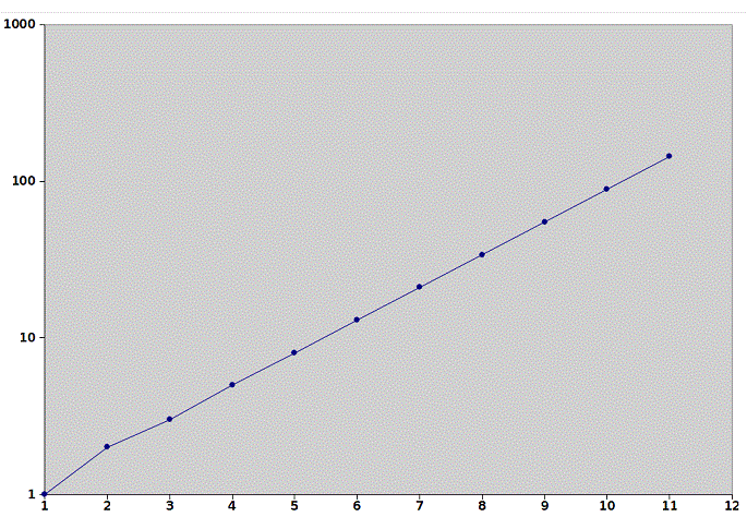
- figure 3. Modeling_Planetary_Distances_log_plot
- figure 3b. Modeling_Planetary_Distances_log_plot_titius_bode
- figure 3c. Modeling_Planetary_Distances_plot_titius_bode_vs_gaussin
- figure 3d. Modeling_Planetary_Distances_gaussin
- figure 3e. Modeling_Planetary_Distances_armenelli
- figure 3f. Modeling_Planetary_Distances_wurm
- figure 4a. Modeling_Planetary_Distances_log_plot_measured_data
- figure 4d. log_plot_Fibonnaci_sequence
- figure 4a.power_law
- figure 4c. power_ln_law
- figure 5.gas_giants
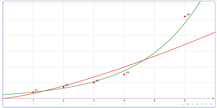
- figure 6. Power law curve fit in red line, e-function curve fit in green line
- figure 7. first_6_points,Power law curve fit in red line, e-function curve fit in green line
- figure 8. power_law
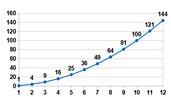
- figure 9.Modeling_Planetary_Distances with the normalized_bohr_atom_1913
- figure 9b.Modeling_Planetary_Distances reference to the normalized_bohr_atom_1913
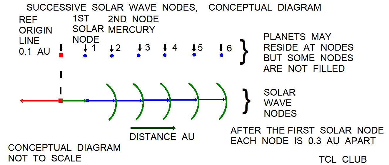
- figure 9c.Modeling_Planetary_Distances_Solar standing_wave
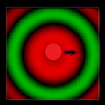
- figure 10. waves, simulation in ripple tank
- figure 11. waves_2, simulation in ripple tank
- References:
- References: Planets, Titius–Bode law
- * Pretty Print Version
- formula from Sven-Ingmar Ragnarsson, 1994
- Appendix: One Liner Procs for Modeling Planetary Distances using Titius-Bode Law and other power laws
- Points for curve fitting
- Hidden Comments Section
Preface
gold 20aug2020 Here are some calculations modeling planetary distances using the Titius-Bode Law. The Titius-Bode Law is primarily of historical interest. But the Titius-Bode is a good exercise in matching the available data.
Introduction
The Titius-Bode Law makes simple assumptions and formulas to model planetary distances by scaling powers of 2. As another accuracy issue, the measured Planetary Distances are identified as non-linear function(s) in the log plots. Reported different velocity estimates in the program and the numerous references involve different assumptions and formulas. In the code, after computing the Titius-Bode output as historical numbers, subsequent formulas are scaled, changed, and different assumptions are changed from the original Titius-Bode formulas.
There are some simple formulas modeling planetary distances using the Titius-Bode Law and other power laws. The Titius-Bode Law is primarily of historical interest. The Titius-Bode law estimated rough distances in Astronomical Units (AU) of Planets from the Sun by scaling powers of 2 in a power law, Johann Elert Bode, pub 1772. There are usually different number assignments for each planet in each formula scheme. The simplest formula number scheme is used here, starting with < Earth = 1... > from Titius-Bode. Although much more is known about planetary distances in modern times, an examination of the original Titius-Bode results gives some fodder for the theory of numerical analysis. The On-Line Encyclopedia of Integer Sequences OEIS refers to the sequences A209257, A003461, and A131500. But the Titius-Bode and other power laws are a good exercise in matching the available data.
Many Distance formulas with different assignment numbers
Here is a summary of Distance formulas and planet assignment numbers for starting the adventure to infinity and beyond. The Titius-Bode formula set < Earth = 1 ... > as number assignment scheme for planets. The Asteroid Ceres is included on most number assignment schemes. Ceres represents the Asteroid belt between Mars and Jupiter. The planet Neptune and dwarf planet Pluto are included on some number assignment schemes. Other planet number schemes are for power laws are available here. The Wurm_formula_1803 was expr {(0.3 + (3.*2.** $nn))*0.1} with the setting < Mercury = -1 ...> But the setting < Mercury = 1 ...> was used by Gaussin (1880) and Armellini (1921) for their power laws. Very interesting, Nicolini transformed planet number scheme in Titius_Bode to < Mercury = 1 ...>, refer to Nicolini. The nicolini_formula_1957 was expr {0.4 + 0.075 * (2. ** $nn)} , $nn=l for Mercury,2,... The Basano_Hughes_formula_1979 was expr {0.285 * (1.523 ** $nn)}, $nn=l for Mercury, 2,... Sven-Ingmar Ragnarsson, 1994, modeled Jupiter and the outer planets to Uranus, separately. See the Ragnarsson paper. For the TCL code, keeping track and comparing these planet assignment numbers is tricky. The Ragnarsson paper used $nn=0 for Jupiter, 2 = Saturn, 3 = Uranus ..... The most successful players separate the non-linear distances into two or three piecewise sections, rather than having a single formula try to cover all the planets and objects.
Many planetary distance papers cited the model of the hydrogen atom developed by Bohr in 1913. The normalized_bohr_atom_1913 formula was expr { 1. * $nn**2 },$nn=1,2,3,4,5 . Here $nn=1 is the first electron orbit.
Revolution Periods and Distance of Planets from the Sun
The Titius–Bode law estimated rough distances in Astronomical Units (AU) of Planets from the Sun by scaling powers of 2, Johann Elert Bode, pub 1772. Although much more known in modern times, an examination of the original Titius–Bode results in AU gives some fodder for the theory of the TCL calculator. For example, Titius–Bode law rated Earth as 1 AU from the Sun and predicted Mars as 1.6 AU. The Bode estimate for Mars was short of the true value 1.676 AU by 4.77 percent error. Using hand calculations, a similar value can be ginned up from the golden ratio, expr { $golden_ratio_constant / 1. } returns 1.618 AU rounded. The golden ratio method is still short of the Mars true distance by 3.6 percent error. Numerous excellent papers have used both the Fibonacci and the golden ratio constants methods to estimate planetary distances from the Sun. The Lombardi paper found the best fit to the Fibonacci constants used the scaling constant < K1 = 55.88 > to get E6 km prediction. Both the Fibonacci and Bode sequences have unassigned slots or skips, due to the Asteroid belt(s) and possible undiscovered bodies. The Asteroid Ceres is representative of Asteroid belt here, but was not known to Bode. Also, both Neptune and Pluto not known to Bode in 1772.
Here is an example of how the Fibonacci method might be used with < K1 = 55.88 > . Astronomer Mary Blagg in 1913 conjectured that if the transplutonian Planet X existed, it might be at ~68 AU from the Sun. The nearest Fibonacci constants are 233 and 377, and unassigned at that. Perhaps, expr { 0.349 * 233. } ;# 81.317 AU for Planet X? The interest in Planet X and the region of 80 AU is not original or new by any means. Schuette suggested a family of comets in the region of 80 AU aphelia, circa 1949. The perihelion of the object Sedna is around 76 AU, reported in 2004. The perihelion of the object 2012 VP is around 80 AU, reported in 2012.
With additional scale factors loaded in the deck, the TCL calculator could use the Fibonacci sequence to output the planetary distances in kilometers and AU. The scale factor for kilometers is 55.88 (*E6). Sample calculation for Planet X was expr { 233. * 55.88 } ;# returns rounded 13000 X 1E6 km The scale factor for AU is expr { 19.2 / 55. } ;# ratio of Uranus returns 0.349 AU/Fi.
Horse Race for Least Squares Fits and Online Curve Fitter
In the horse race of fitting formulas, a least squares method was fit to the curve with some known initial points either with the first 6 planets or 9 planets, if Pluto or Ceres included. Other fits to the curve can be tried from an online curve fitter, using the least squares method. A Gaussian bell curve was not a good fit to the eyeball. The linear fit or stick fit was tried. The linear slope can be defined from simple points.
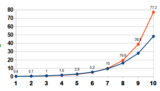
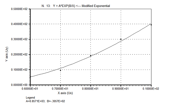
Candidate models of fit include 1) Weibull growth curve, 2) Ratkowsky Model, 3) power law and 4) exponential law, which appear winners of field with more than 208 entries for fitting functions. The fitting algorithm for points was available to double precision, E-14. But obviously, such precision was not necessary with the 3 significant figures in reported JPL measured data. Some calculations appear defaulted to single precision, E-7. The tabled chi results were from 208 equations of 2 parameters (2P) or 2 terms (t2), from the non-linear curve fit algorithm (NLCF). Undoubtedly, this computer task would be hundreds of man-hours in paper calculations, but done automatically on the computer in three seconds or less. Trig functions are trivial results in this search, but leaving available in table, in case results jog memory. Also, there was a really nice piecewise cubic spline fit for 9 planets, but not sure how to wrap in code. One can see how the power laws or doubling rules like the Titius-Bode formula are breaking down beyond Jupiter and Uranus. See figures 6 and 7.
In the horse race of fitting formulas, a least squares method was fit to the curve with some known initial points either with the first 6 planets or 9 planets, if Pluto or Ceres included. Other fits to the curve can be tried from an online curve fitter, using the least squares method. Candidate models of fit include 1) Y=A*EXP(((X-B)**2)/C) exponential 2) Y = A*(B**(1/X))*X**C <--- Mod Hoerl , 2) Y = A*X+B*X**2+C*X**3 <--- 3nd order polynomial, 3) Y = A*(B**(1/X))*X**C <--- Mod Hoerl, and 4) Y = A*X**B+C <--- 1 pow + c, which appear winners of field with more than 208 entries for fitting functions. For inclusion in the horse race of fitting formulas, the classic sigmoidal functions were estimated like the Weibull growth curve, Gompetrz growth curve, and Ratkowsky Model growth curve. For the raw Planet Distances, the online fitter reported that the std of measured X values was 3.022 and avg X value was 5.555. The std of measured Y values was 13.655 and avg Y value was 11.902. The Weibull growth curve < a - b*exp(-c*x**d)> had a standard error of 4.25E-01 and a correlation coefficient of 9.99E-01. The Ratkowsky Model had a standard error of 5.29E-01 and a correlation coefficient of 9.99E-01. The Gompertz growth curve standard error of 1.96E+00 and correlation coefficient of 9.93E-01. The Logistic Power function had an standard error of 8.07E-01 and a correlation coefficient of 9.98E-01. Of most interest for comparison with the historic Titius-Bode power law, the Modified Power function <y=a*C**x> had standard error of 2.01E+00 and a correlation coefficient of 9.91E-01.
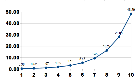
The autofitter found a = 5.14E-01 and b = 1.55E+00 for the Modified Power function <y=a*C**x>, which was close to the Armellini formula for planetary distances. In 1921, G. Armellini suggested a planetary distance formula, equivalent to <y = 0.2792 x 1.53**n> . Other authors have suggested 1.73 or, 1.842, for the C term in a planetary distance power function <y=a*b**x>. The Modified Power function error is at 5 percent of the Y axis, which is at the non-significant borderline level generally cited. The Weibull growth curve should fit the Y axis with a 1 percent error. In these growth functions, the Levenberg-Marquardt (L-M) algorithm was used with double precision C's.
Considerations for Code and Titius-Bode formulas into TCL code
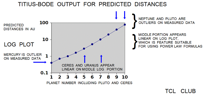
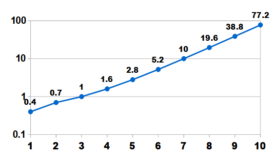
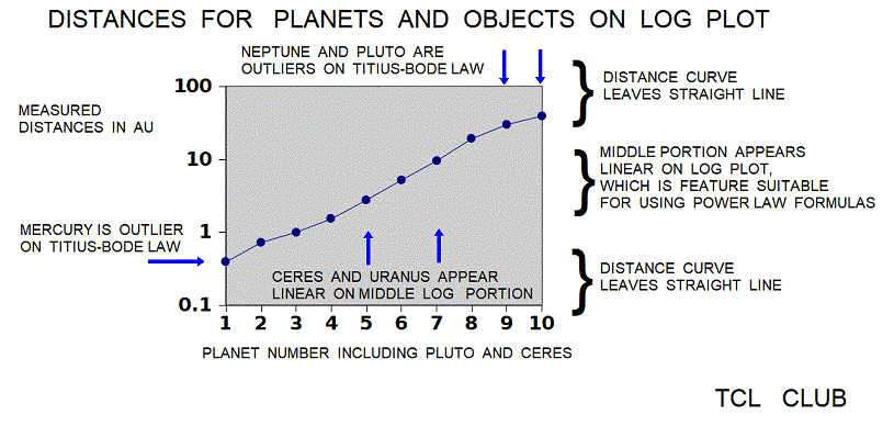
For fitting power law formulas to the measured data, Mercury, Neptune, and Pluto are outlier points. Ceres and Uranus from the measured data appear on the middle portion in the log chart of the measured data. The linear appearance of the middle portion feature is suitable for using power law formulas. The TCL calculator uses planet assignment numbers from 1 to 10, including the Pluto dwarf planet and the Ceres asteriod.
Pushbutton Operation
For the push buttons, the recommended procedure is push testcase and fill frame, change first three entries etc, push solve, and then push report. Report allows copy and paste from console. For testcases in a computer session, the eTCL calculator increments a new testcase number internally, eg. TC(1), TC(2) , TC(3) , TC(N). The testcase number is internal to the calculator and will not be printed until the report button is pushed for the current result numbers. The current result numbers will be cleared either on the next clear button or on the next solve button. All results will be lost on program exit, unless the report text is saved from the report screen on console.
Conclusions
In the horse race of fitting formulas, a least squares method was fit to the curve with some known initial points either with the first 6 planets or 9 planets, if Pluto or Ceres included. Other fits to the curve can be tried from an online curve fitter, using the least squares method. Candidate models of fit include 1) Y=A*EXP(((X-B)**2)/C) exponential 2) Y = A*(B**(1/X))*X**C <--- Mod Hoerl , 2) Y = A*X+B*X**2+C*X**3 <--- 3nd order polynomial, 3) Y = A*(B**(1/X))*X**C <--- Mod Hoerl, and 4) Y = A*X**B+C <--- 1 pow + c, which appear winners of field with more than 208 entries for fitting functions. The tabled chi results were from 208 equations of 2 parameters (2P) or 2 terms (t2), from the non-linear curve fit algorithm (NLCF). Undoubtedly, this computer task would be hundreds of man-hours in paper calculations, but done automatically on the computer in three seconds or less. In the code, after computing the Titius-Bode output as historical numbers, subsequent formulas are scaled, changed, and different assumptions are changed from the original Titius-Bode formulas.
The set of measured planet distances is a non-linear function, which possibly should be modeled in three sections. From the log plots, there appears to be a sine wave or sigmoidal growth function component in the measured planet distances, meaning non-linear S-curve in slang. Again from the log plots, one can see how the power laws or doubling rules like the Titius-Bode formula are breaking down beyond Jupiter and Uranus. The Ragnarsson paper in 1994 showed fair results in modeling Jupiter and the outer planets as a separate section.
| Table : Est. Distance of Planets from Fibonacci and Bode Rules | printed in tcl wiki format | |||||||
|---|---|---|---|---|---|---|---|---|
| sources >> | JPL | JPL | Fibonacci constants | Lombardi Paper | Lombardi Paper | Wikipedia | Wikipedia | comments |
| quantity | real measured AU, semi_major axis | real measured 10E6 km, semi_major axis | Fibonacci constants | Fibonacci * 55.88, 10E6 km Prediction | Titius-Bode number | Titius-Bode AU Prediction | Real Measured AU , semi_major axis | comments, if any |
| Sun | 0 | 0 | Sun not assigned value in Fibonacci and Bode Rules | |||||
| Mercury | 0.39 | 57.9 | 1 | 55.8 | 4 | 0.4 | 0.39 | |
| Venus | 0.723 | 108.2 | 2 | 111.6 | 7 | 0.7 | 0.72 | |
| Earth | 1 | 149.6 | 3 | 167.4 | 10 | 1 | 1 | Earth assigned unit 1 AU in Bode Rules |
| Mars | 1.524 | 227.9 | 5 | 279 | 16 | 1.6 | 1.52 | |
| Ceres | 2.767 | 265.3 | 8 | 446.4 | 28 | 2.8 | 2.77 | Asteroid belt |
| Jupiter | 5.203 | 778.3 | 13 | 725.4 | 52 | 5.2 | 5.2 | |
| Jupiter clearance belt | 21 | 1171.8 | Jupiter clearance belt | |||||
| Saturn | 9.539 | 1427 | 34 | 1897.2 | 100 | 10 | 9.55 | |
| Uranus | 19.18 | 2871 | 55 | 3069 | 196 | 19.6 | 19.22 | |
| Neptune | 30.07 | 4497.1 | 89? | 4966.2 | 388? | 38.8? | 30.11 | Bodes Law breaks down for Neptune and Pluto. Confusing references. |
| Pluto (avg) | 39.482 | 5906.38 | 144? | 8035.2? | 772? | 77.20? | 39.54 | Pluto is not considered a planet, currently. Bodes Law breaks down for Neptune and Pluto. Confusing references. |
| Note | several sources | Wikipedia | Jpl | Lombardi Paper | ||||
| Note | Neptune, Pluto, & Ceres were not known to Bode | |||||||
| Note | Ceres representative of Asteroid belt here | |||||||
| Note | Bodes Law breaks down for Neptune and Pluto, confusing references | Opinion: Bode Number assignment for N&P uncertain here. |
Testcases Section
In planning any software, it is advisable to gather a number of testcases to check the results of the program.
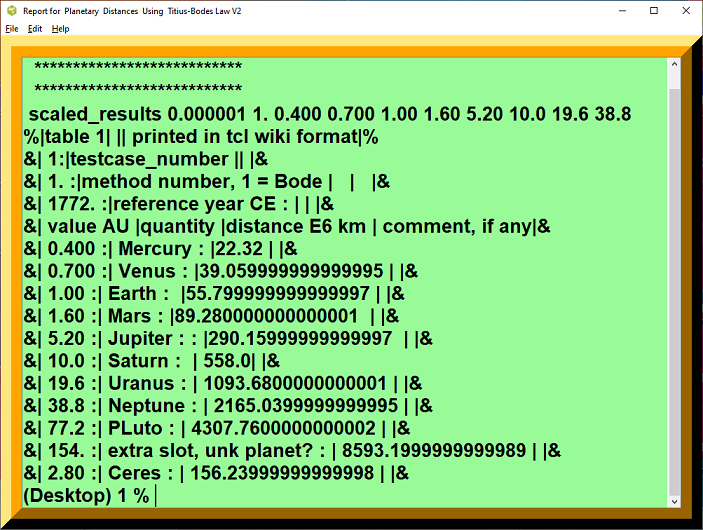
Testcase 1, Planet distances in AU
| Testcase 1 | printed in tcl wiki format | ||
|---|---|---|---|
| 1: | testcase_number | ||
| 1. : | method number, 1 = Bode | ||
| 1772. : | reference year CE : | ||
| value AU | quantity | distance E6 km | comment, if any |
| 0.400 : | Mercury : | 22.32 | Bodes Law breaks down for Mercury |
| 0.700 : | Venus : | 39.059 | |
| 1.00 : | Earth : | 55.79 | Earth set to one in Bodes Law |
| 1.60 : | Mars : | 89.280 | |
| 5.20 : | Jupiter : : | 290.159 | |
| 10.0 : | Saturn : | 558.0 | |
| 19.6 : | Uranus : | 1093.68 | |
| 38.8 : | Neptune : | 2165.039 | Bodes Law breaks down for Neptune and Pluto. |
| 77.2 : | Pluto : | 4307.76 | Pluto is not considered a planet, currently. Bodes Law breaks down for Neptune and Pluto. |
| 154. : | extra slot, unk planet? : | 8593.19 | |
| 2.80 : | Ceres : | 156.23 | represents Asteroid belt here |
  Console wrapper for solution proc
  ***************************
  ***************************
 scaled_results 0.000001 1. 0.400 0.700 1.00 1.60 5.20 10.0 19.6 38.8
Screenshots Section
figure 1. screenshot
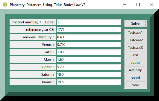
figure 2. Calculator_report
figure 3. Modeling_Planetary_Distances_log_plot
figure 3b. Modeling_Planetary_Distances_log_plot_titius_bode
figure 3c. Modeling_Planetary_Distances_plot_titius_bode_vs_gaussin
figure 3d. Modeling_Planetary_Distances_gaussin
figure 3e. Modeling_Planetary_Distances_armenelli
figure 3f. Modeling_Planetary_Distances_wurm
figure 4a. Modeling_Planetary_Distances_log_plot_measured_data
figure 4d. log_plot_Fibonnaci_sequence
figure 4a.power_law
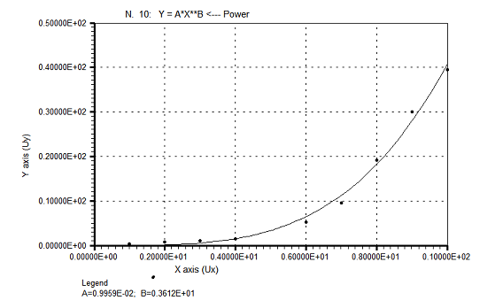
figure 4c. power_ln_law
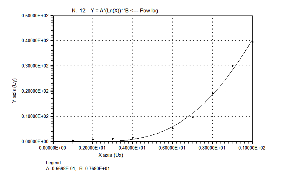
figure 5.gas_giants
figure 6. Power law curve fit in red line, e-function curve fit in green line
Power law curve fit in red line
Power law parameter
a=0.182490688
b=2.104691172
Power law
y=a⋅xb=0.182490688⋅x2.104691172
Standard deviation
σ=7.340978516
e-function curve fit in green line
Parameter of the fitted e-function
a=0.535853432
b=0.218240397
The e-Function
f(x)=b⋅ea⋅x=0.218240397⋅e0.535853432⋅x
Standard deviation
σ=17.056378115
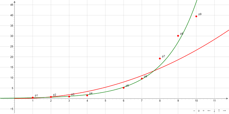
figure 7. first_6_points,Power law curve fit in red line, e-function curve fit in green line
figure 8. power_law
figure 9.Modeling_Planetary_Distances with the normalized_bohr_atom_1913
figure 9b.Modeling_Planetary_Distances reference to the normalized_bohr_atom_1913
figure 9c.Modeling_Planetary_Distances_Solar standing_wave
figure 10. waves, simulation in ripple tank
photo credit, ripple tank at falstad.com website.
Golden_Ratio_waves_ripple_tank
figure 11. waves_2, simulation in ripple tank
photo credit, ripple tank at falstad.com website.
References:
- Wikipedia search engine < Titius Bode >
- Wikipedia search engine < Golden Mean >
- Wikipedia search engine < Programming Examples >
- Google search engine < vaporware >
References: Planets, Titius–Bode law
- wikipedia.org/wiki/Titius Bode law
- Article: All Solar system periods fit
- the Fibonacci series and the Golden Ratio.
- Posted: February 20, 2013 by tallbloke
- The Golden Mean In The Solar System,
- Oreste W. Lombard I And Margaret A. Lombardi
- On a Suggested Substitute for Bode’s Law. By M. A. Blagg.
- Communicated by Professor H. B. Turner.
- Planetary distances: a new simplified model
- Sven-Ingmar Ragnarsson, 1994
- Fibonacci Series In The Solar System
- Captain B. A. Read, Canada
- A postulate leading to the Titius-Bode law
- R. Louise
- www.jpl.nasa.gov/edu/pdfs/scaless_reference.pdf
- Schuette, C. H., "Two new families of comets", Pop. Astron. 57, 176-82
- (1949); "Drei weitere Mitglieder der Transplutokometenfamilie", Acta
- Astronomica 15, 11-13 (1965).
- Bode’s Law And Spiral Structure In Nebulae
- By William Sutherland
- A Sedna-like body with a perihelion of 80
- astronomical units
- Chadwick A. Trujillo, Scott S. Sheppard
- Searching For Sedna’s Sisters: Exploring The Inner Oort Cloud
- Megan Schwamb with Advisor: Mike Brown
- A new object at the edge of our Solar System discovered
- by Carnegie Institution for Science
- Modeling Celestial Mechanics Using the Fibonacci Number,
- Robert G. Sacco, 2019
- A Supposed New Law For Planetary Distances, letter,
- Ennio Badolati, 1982, several approaches cited
- Munini and Armellini (1978) , d = 0.283 x 1.52**n, sequence < n = 1,2,... 12 >
- 1880 Gaussin, d~ = 0.2099 x 1.7226**n, (n = 1,2... 9)
- tester formula, d = $K1 x 1.842**n, sequence < n = 1,2,... 12 >
- Planetary distances: a new simplified model
- Sven-Ingmar Ragnarsson
Caption outline on plots. distance curve Leaves straight line middle portion appears Linear on log plot, Which is feature suitable For using power law formulas Mercury is outlier On measured data Distance curve Leaves straight le Neptune and pluto are Outliers on measured data Ceres and uranus appear Linear on middle log portion Titius-Bode output for predicted distances tcl club Planet number including Pluto and Ceres Distance curve Leaves straight line Distance curve Leaves straight line Middle portion appears Linear on log plot, Which is feature suitable For using power law formulas Mercury is outlier On titius-bode law Distance curve Leaves straight le Neptune and pluto are Outliers on titius-bode law Ceres and uranus appear Linear on middle log portion {distances for planets and objects on log plot } Tcl club } Planet number including Pluto and Ceres
Appendix TCL programs and scripts
* Pretty Print Version
        #  pretty print from autoindent and ased editor occurrence
        #  Planetary  Distances  Using  Titius-Bodes Law V2 calculator
        #  written on Windows 10
        #  working under TCL version 8.6
        #  gold on TCL Club, 10jul2021
        package require Tk
        package require math::numtheory
        namespace path {::tcl::mathop ::tcl::mathfunc math::numtheory }
        set tcl_precision 17
        frame .frame -relief flat -bg aquamarine4
        pack .frame -side top -fill y -anchor center
        set names {{} { method number, 1 = Bode :} }
        lappend names {reference year CE: }
        lappend names {answers:  Mercury  : }
        lappend names { Venus  : }
        lappend names { Earth  : }
        lappend names { Mars  : }
        lappend names { Jupiter  : }
        lappend names { Saturn  : }
        lappend names { Uranus  : }
        foreach i {1 2 3 4 5 6 7 8 9} {
            label .frame.label$i -text [lindex $names $i] -anchor e
            entry .frame.entry$i -width 35 -textvariable side$i
            grid .frame.label$i .frame.entry$i -sticky ew -pady 2 -padx 1 }
        proc about {} {
            set msg "Calculator for  Planetary  Distances  Using  Titius-Bodes Law V2
            from TCL WIKI,
            written on TCL 8.6 "
            tk_messageBox -title "About" -message $msg }
        proc self_help {} {
            set msg "Calculator for  Planetary  Distances  Using  Titius-Bodes Law V2
            from TCL ,
            #  self help listing
            #  1 given  follow.
            1) method  N1
            2) Reference year
            #  This calculator uses the Titius-Bodes Law
            #  to predict Planetary Distances in AU.
            #  For comparison, TCL code may include redundant paths & formulas.
            #  The TCL calculator normally uses modern
            #  units  for convenience to modern users and textbooks.
            #  Any convenient and consistent in/output units might be used
            #  like inches, feet, nindas, cubits, or dollars to donuts.
            #  Recommended procedure is push testcase and fill frame,
            #  change first three entries etc, push solve,
            #  and then push report. Report allows copy and paste
            #  from console to conventional texteditor. For testcases
            #  testcase number is internal to the calculator and
            #  will not be printed until the report button is pushed
            #  for the current result numbers.
            #  Use one line errorx proc to estimate percent errors.
            #  errorx proc is used in the report window (console).
            #  Additional significant figures are used to check
            #  the TCL program, not to infer the accuracy
            #  of inputs and product reports.
            Conventional text editor formulas or  grabbed from internet
            screens can be pasted into green report console.
            Try copy and paste following into green screen console
            set answer \[* 1. 2. 3. 4. 5. \]
            returns  120
            #  gold on  TCL Club, 10jul2021 "
            tk_messageBox -title "self_help" -message $msg }
        proc precisionx {precision float}  {
            #   tcl:wiki:Floating-point formatting, <AM>
            #  select numbers only, not used on every number.
            set x [ expr {round( 10 ** $precision * $float) / (10.0 ** $precision)} ]
            #   rounded or clipped to nearest 5ird significant figure
            set x [ format "%#.3g" $x ]
            return $x
        }
        #  Use one line errorx proc to estimate percent errors
        #  errorx proc is used in the report window (console)
        proc errorx  {aa bb} {expr { $aa > $bb ?   (($aa*1.)/$bb -1.)*100. : (($bb*1.)/$aa -1.)*100.}}
        proc titius_bode_law  {aa } {expr { (4. + 3 * 2**$aa)*.1 } }
        proc calculate {     } {
            global answer2
            global side1 side2 side3 side4 side5
            global side6 side7 side8 side9 k1
            global side10 side11 side12 side13
            global testcase_number
            incr testcase_number
            #  scaling constant K1
            set k1 55.8
            set side3 [precisionx 2 [ titius_bode_law -1]]
            set side4 [precisionx 2 [ titius_bode_law 0]]
            set side5 [precisionx 2 [ titius_bode_law 1]]
            set side6 [precisionx 2 [ titius_bode_law 2]]
            set side7 [precisionx 2 [ titius_bode_law 4]]
            set side8 [precisionx 2 [ titius_bode_law 5]]
            set side9 [precisionx 2 [ titius_bode_law 6]]
            set side10 [precisionx 2 [ titius_bode_law 7]] #  Neptune
            set side11 [precisionx 2 [ titius_bode_law 8]] #  Pluto
            set side12 [precisionx 2 [ titius_bode_law 9]] #  extra Bode slot, unk planet?
            set side13 [precisionx 2 [ titius_bode_law 3]] #  Ceres
            set scaled_results [list 0.000001 $side1 $side3 $side4 $side5 $side6 $side7 $side8 $side9 $side10]
            puts " scaled_results $scaled_results "
             }
        proc fillup {aa bb cc dd ee ff gg hh ii} {
            .frame.entry1 insert 0 "$aa"
            .frame.entry2 insert 0 "$bb"
            .frame.entry3 insert 0 "$cc"
            .frame.entry4 insert 0 "$dd"
            .frame.entry5 insert 0 "$ee"
            .frame.entry6 insert 0 "$ff"
            .frame.entry7 insert 0 "$gg"
            .frame.entry8 insert 0 "$hh"
            .frame.entry9 insert 0 "$ii"
             }
        proc clearx {} {
            foreach i {1 2 3 4 5 6 7 8 9 } {
                .frame.entry$i delete 0 end } }
        proc reportx {} {
            global side1 side2 side3 side4 side5
            global side6 side7 side8 side9 k1
            global side10 side11 side12 side13
            global testcase_number
            console show;
            puts "%|table $testcase_number| || printed in tcl wiki format|% "
            puts "&| $testcase_number:|testcase_number || |&"
            puts "&| $side1 :|method number, 1 = Bode |   |   |&"
            puts "&| $side2 :|reference year CE : | | |& "
            puts "&| value AU |quantity |distance E6 km | comment, if any|& "
            puts "&| $side3 :| Mercury : |[* $side3  $k1 ] | |& "
            puts "&| $side4 :| Venus : |[* $side4  $k1 ] | |& "
            puts "&| $side5 :| Earth :  |[* $side5  $k1 ] | |&"
            puts "&| $side6 :| Mars : |[* $side6  $k1 ]  | |&"
            puts "&| $side7 :| Jupiter : : |[* $side7  $k1 ]  | |&"
            puts "&| $side8 :| Saturn :  | [* $side8  $k1 ]| |&"
            puts "&| $side9 :| Uranus : | [* $side9  $k1 ] | |&"
            puts "&| $side10 :| Neptune : | [* $side10  $k1 ] | |&"
            puts "&| $side11 :| Pluto : | [* $side11  $k1 ] | |&"
            puts "&| $side12 :| extra slot, unk planet? : | [* $side12  $k1 ] | |&"
            puts "&| $side13 :| Ceres : | [* $side13  $k1 ] | |&"
            }
        frame .buttons -bg aquamarine4
        ::ttk::button .calculator -text "Solve" -command { calculate   }
        ::ttk::button .test2 -text "Testcase1" -command {clearx;fillup 1. 1772. 0.40  0.70  1.0  1.6  5.2  10. 19.6}
        ::ttk::button .test3 -text "Testcase2" -command {clearx;fillup 1. 1772. 0.40  0.70  1.0  1.6  5.2  10. 19.6}
        ::ttk::button .test4 -text "Testcase3" -command {clearx;fillup 1. 1772. 0.40  0.70  1.0  1.6  5.2  10. 19.6}
        ::ttk::button .clearallx -text clear -command {clearx }
        ::ttk::button .about -text about -command {about}
        ::ttk::button .self_help -text self_help -command {self_help }
        ::ttk::button .cons -text report -command { reportx }
        ::ttk::button .exit -text exit -command {exit}
        pack .calculator  -in .buttons -side top -padx 10 -pady 5
        pack  .clearallx .cons .self_help .about .exit .test4 .test3 .test2   -side bottom -in .buttons
        grid .frame .buttons -sticky ns -pady {0 10}
               . configure -background aquamarine4 -highlightcolor brown -relief raised -border 30
        wm title . " Planetary  Distances  Using  Titius-Bodes Law V2"
        # end of working deck
        # add cosmetics below to bottom of file
        console eval {.console config -bg palegreen}
        console eval {.console config -font {fixed 20 bold}}
        console eval {wm geometry . 40x20}
        console eval {wm title . " Report for  Planetary  Distances  Using  Titius-Bodes Law V2  "}
        console eval {. configure -background orange -highlightcolor brown -relief raised -border 30}
        puts "  Console wrapper for solution proc"
        puts "  ***************************"
        puts "  ***************************"
formula from Sven-Ingmar Ragnarsson, 1994
  2 tiered formula from Sven-Ingmar Ragnarsson, 1994
  expr { 2.825/5  } ;# 0.565   Mercury badly off
  expr { 2.825/4  } ;# 0.70625 Venus
  expr { 2.825/3  } ;# 0.9416  Earth
  expr { 2.825/2  } ;# 1.412  Mars
  expr { 2.825/1  } ;# 2.825  Ceres
  expr { 5.203*(((5./2.)**(2./3.))**0)  } ;# 5.203  Jupiter
  expr { 5.203*(((5./2.)**(2./3.))**1)  } ;# 9.584  Saturn
  expr { 5.203*(((5./2.)**(2./3.))**2)  } ;# 17.653 Uranus
  expr { 5.203*(((5./2.)**(2./3.))**3)  } ;# 32.51875 Neptune? badly off
  expr { 5.203*(((5./2.)**(2./3.))**4)  } ;# 59.9 ?  PLuto? badly off
Appendix: One Liner Procs for Modeling Planetary Distances using Titius-Bode Law and other power laws
     #  for starting the adventure  to infinity and beyond.
     #   Titius-Bode set < Earth = 1 ... > as number assignment scheme for planets
     #  The Asteriod Ceres is included on most number assignment schemes
     #  Ceres represents the Asteriod belt between Mars and Jupiter.
     #  The dwarf planet Pluto  is included on most number assignment schemes.
     proc titius_bode_law_1772  {aa } {expr { (4. + 3 * 2**$aa)*.1 } }  #  #  $nn=l for Earth,2,...
     #  Other planet number schemes are for power laws are available here, < Mercury = 1 ...>
     #  from Gaussin (1880) and Armellini (1921)
     proc gaussin_formula_1880  {nn} {expr {0.2099 * (1.7226 ** $nn)} } #  $nn=l for Mercury,2,...9
     proc armellini_formula_1921  {nn} {expr {0.283 * (1.53 ** $nn)} }  #  $nn=l for Mercury,2,...11
     #  very interesting, Nicolini transformed planet number scheme in  Titius_Bode
     #  to < Mercury = 1 ...>, refer to Nicolini
     proc nicolini_formula_1957  {nn} {expr {0.4 + 0.075 * (2. ** $nn)} }  #  $nn=l for Mercury,2,...
     proc basano_hughes_formula_1979  {nn} {expr {0.285 * (1.523 ** $nn)} } #  $nn=l for Mercury, 2,...
     #  Sven-Ingmar Ragnarsson, 1994, modeled Jupiter and the outer planets to Uranus, separately.
     #  See the  Ragnarsson paper, setting these planet assignment numbers is tricky.
     #  $nn=0 for Jupiter, 2 = Saturn, 3 = Uranus ....
     proc ragnarsson_formula_1979  {nn} {expr {5.203*(((5./2.)**(2./3.))**$nn) )} } #  $nn=0 for Jupiter, 2 = Saturn,...
     proc list_integers { aa bb} { for {set i 1} {$i<=$bb} {incr i} {lappend boo [* 1. $i ] [*  $i  1.]};return $boo}
     #  usage, list_integers 1 10
     #  set answer_list_integers = [list 1.0  1.0 2.0 2.0 3.0 3.0 4.0 4.0 5.0 5.0 6.0 6.0 7.0 7.0 8.0 8.0 9.0 9.0 10.0 10.0 ]
     proc list_titius_bode  { aa bb} { for {set i 1} {$i<=$bb} {incr i}    {lappend boo [* 1. $i ] [expr { (4. + 3. * 2**$i)*.1}]};if {$i > $bb} {return $boo}}
     #  Usage   list_titius_bode 1 6
     #  set answer [ list 1.0 1.0 2.0 1.6 3.0 2.8 4.0 5.2 5.0 10.0 6.0 19.6]
      proc list_gaussin_formula  { aa bb} { for {set ii 1} {$ii<=$bb} {incr ii} {lappend boo [* 1. $ii ] [expr {0.2099 * (1.7226 ** $ii)} ]};if {$ii > $bb} {return $boo}}
      #  Usage   list_gaussin_formula 1 6
      #  set answer_gaussin [ list 1.0 0.36  2.0 0.62  3.0 1.07  4.0 1.84  5.0 3.18  6.0 5.48 ]
      proc list_armellini_formula  { aa bb} { for {set ii 1} {$ii<=$bb} {incr ii}    {lappend boo [* 1. $ii ] [expr {0.283 * (1.53  ** $ii)}]};if {$ii > $bb} {return $boo}}
      #  Usage  list_armellini_formula 1 7
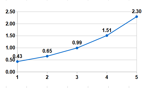
      #  set answer_armellini [  1.0 0.43 2.0 0.66 3.0 1.013 4.0 1.55 5.0 2.37 6.0 3.63  7.0 5.55 ]
Points for curve fitting
         1                0.39
         2                0.723
         3                1.
         4                1.524
         6                5.203
         7                9.539
         8                19.18
         9                30.07
        10                39.482
Hidden Comments Section
Please include your wiki MONIKER and date in your comment with the same courtesy that I will give you. Thanks, gold 12Aug2020
gold 9/27/2021. Switched some comment signs ;# to #. This a big file. Check earlier editions, if not compatible. Maybe obvious, but this page was written on Windows10 Tcl ports including ActiveTCL. I assume reader can cut and paste on screen, what the reader needs, and tootle on to his own project and own contribution pages to the TCL Wiki.
| Category Numerical Analysis | Category Toys | Category Calculator | Category Mathematics | Category Example | Toys and Games | Category Games | Category Application | Category GUI |
