Sales Optimal Lot Order Size and eTCL Slot Calculator Demo Example
This page is under development. Comments are welcome, but please load any comments in the comments section at the bottom of the page. Please include your wiki MONIKER and date in your comment with the same courtesy that I will give you. Aside from your courtesy, your wiki MONIKER and date as a signature and minimal good faith of any internet post are the rules of this TCL-WIKI. Its very hard to reply reasonably without some background of the correspondent on his WIKI bio page. Thanks, gold 12DEC2018
- Introduction
- Appendix Code
- Draft Figures, ASCII Diagrams
- figure. OPTIMAL LOT ORDER SIZE: BASIC CONCEPT
- figure. ECONOMIC ORDER QUANTITY FORMULA
- figure. eTCL OPTIMAL LOT ORDER SIZE CALCULATOR DEMO
- figure. TOTAL COST CURVE FOR LOT SIZING
- figure. SENSITIVITY ANALYSIS IN LOT SIZING
- figure. eTCL CONSOLE EXAMPLE FOR OPTIMAL LOT SIZE
- figure. WILSON LOT ORDER SIZE (EOQ) FORMULA: CORE IDENTITY
- figure. EOQ COST CURVE: ORDERING vs HOLDING vs TOTAL
- figure. NUMBER OF ORDERS AND REORDER POINT
- figure. CALCULATE PROC: FORMULA FLOW
- figure. TESTCASE RESULTS SUMMARY (3 testcases)
- figure. EOQ ASSUMPTIONS AND REAL-WORLD LIMITATIONS
- figure. eTCL SLOT CALCULATOR: GUI LAYOUT
- figure. PSEUDOCODE AND EQUATIONS SUMMARY
- figure. OVERALL PROGRAM FLOW
- figure. SUMMARY: OPTIMAL LOT ORDER SIZE
- Comments Section
Introduction
gold Here are some TCL calculations for the Sales Optimal Lot Order Size The inventory_cost equals (ordering_cost*units_sold)/order_quantity + (unit_price*units_sold +holding_cost*order_quantity/2. The optimal order_quantity equals sqrt < (2.*ordering_cost*units_sold)/holding_cost>. In the TCL calculator the holding_cost is calculated over a time period, usually 7 days. The holding_cost is dollars per unit per time interval. Most of the testcases involve experiments or models, using assumptions and rules of thumb.
The inventory_cost equals (ordering_cost*units_sold)/order_quantity + (unit_price*units_sold +holding_cost*order_quantity/2. The optimal order_quantity equals sqrt <(2.*ordering_cost*units_sold)/holding_cost>. In the calculator the holding_cost is calculated over a time period, usually 7 days. The holding_cost is dollars per unit per time interval.
Pseudocode and Equations
  price? = raw materials + labor  +  profit
  price? = raw materials + heat process
  price? = raw materials + labor
  average price per unit  = revenue  / units sold
Testcases Section
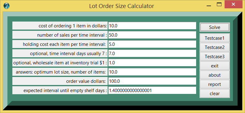
In planning any software, it is advisable to gather a number of testcases to check the results of the program. The math for the testcases can be checked by pasting statements in the TCL console. Aside from the TCL calculator display, when one presses the report button on the calculator, one will have console show access to the capacity functions (subroutines).
Testcase 1
| table 1 | printed in | tcl wiki format |
|---|---|---|
| quantity | value | comment, if any |
| testcase number: | 1 | |
| 10.0 : | cost of ordering 1 item in dollars | |
| 50.0 : | number of sales per time interval | |
| 5.0 : | holding cost per time interval | |
| 7.0 : | time interval days usually 7 | |
| 1.0 : | inventory item trial value | |
| 10.0: | answers: lot size | |
| 100.0 : | order value dollars | |
| 1.40 : | expected interval for empty shelf days | |
| 10.0 : | discounted inventory total dollars | trial item usually 1 d. |
Testcase 2
| table 2 | printed in | tcl wiki format |
|---|---|---|
| quantity | value | comment, if any |
| testcase number: | 2 | |
| 100.0 : | cost of ordering 1 item in dollars | |
| 1000.0 : | number of sales per time interval | |
| 10.0 : | holding cost per time interval | |
| 7.0 : | time interval days usually 7 | |
| 1.0 : | inventory item trial value | |
| 100.0: | answers: lot size | |
| 10000.0 : | order value dollars | |
| 0.700 : | expected interval for empty shelf days | |
| 100.0 : | discounted inventory total dollars | trial item usually 1 d. |
Testcase 3
| table 3 | printed in | tcl wiki format |
|---|---|---|
| quantity | value | comment, if any |
| testcase number: | 3 | |
| 10.0 : | cost of ordering 1 item in dollars | |
| 100.0 : | number of sales per time interval | |
| 10.0 : | holding cost per time interval | |
| 7.0 : | time interval days usually 7 | |
| 1.0 : | inventory item trial value | |
| 10.0: | answers: lot size | |
| 100.0 : | order value dollars | |
| 0.700 : | expected interval for empty shelf days | |
| 10.0 : | discounted inventory total dollars | trial item usually 1 d. |
Screenshots Section
figure 1.
References:
- Stat
Appendix Code
appendix TCL programs and scripts
        # pretty print from autoindent and ased editor
        # Wilson lot order size sales calculator
        # written on Windows XP on eTCL
        # working under TCL version 8.5.6 and eTCL 1.0.1
        # gold on TCL WIKI, 10oct2014
        # comment follows from gold, 12Dec2018
        # pretty print from autoindent and ased editor
        # Wilson Lot Order Size Sales Calculator V2
        # written on Windows XP on TCL
        # working under TCL version 8.6
        # Revamping older program from 2014.
        package require Tk
        namespace path {::tcl::mathop ::tcl::mathfunc}
        frame .frame -relief flat -bg aquamarine4
        pack .frame -side top -fill y -anchor center
        set names {{} {cost of ordering 1 item in dollars:} }
        lappend names {number of sales per time interval :}
        lappend names {holding cost each item per time interval: }
        lappend names {optional, time interval days usually 7 :}
        lappend names {optional, wholesale item at inventory trial $1 :}
        lappend names {answers: optimum lot size, number of items: }
        lappend names {order value dollars: }
        lappend names {expected interval until empty shelf days :}
        foreach i {1 2 3 4 5 6 7 8} {
            label .frame.label$i -text [lindex $names $i] -anchor e
            entry .frame.entry$i -width 35 -textvariable side$i
            grid .frame.label$i .frame.entry$i -sticky ew -pady 2 -padx 1 }
        proc about {} {
            set msg "Calculator for Lot Order Size
            from TCL ,
            # gold on  TCL Club, 12Dec2018 "
            tk_messageBox -title "About" -message $msg }
        proc self_help {} {
            set msg " Lot Order Size V2
            from TCL Club ,
            # self help listing
            # problem, Lot Order Size V2
            # 3 givens follow.
            1) cost of ordering 1 item in dollars:
            2) number of sales per time interval:
            3) holding cost each item per time interval:
            4) optional, time interval days usually 7:
            5) optional, wholesale item at inventory trial $1:
            # Recommended procedure is push testcase
            # and fill frame,
            # change first three entries etc, push solve,
            # and then push report.
            # Report allows copy and paste
            # from console to conventional texteditor.
            # For testcases, testcase number is internal
            # to the calculator and will not be printed
            # until the report button is pushed
            # for the current result numbers.
            # >>> copyright notice <<<
            # This posting, screenshots, and TCL source code is
            # copyrighted under the TCL/TK license terms.
            # Editorial rights and disclaimers
            # retained under the TCL/TK license terms
            # and will be defended as necessary in court.
            Conventional text editor formulas
            or  formulas grabbed from internet
            screens can be pasted into green console.
            # gold on  TCL Club, 12Dec2018 "
            tk_messageBox -title "Self_Help" -message $msg }
        proc calculate {     } {
            global answer2
            global side1 side2 side3 side4 side5
            global side6 side7 side8
            global discounted_inventory
            global testcase_number
            incr testcase_number
            set side1 [* $side1 1. ]
            set side2 [* $side2 1. ]
            set side3 [* $side3 1. ]
            set side4 [* $side4 1. ]
            set side5 [* $side5 1. ]
            set side6 [* $side6 1. ]
            set side7 [* $side7 1. ]
            set side8 [* $side8 1. ]
            set cost_order  $side1
            set number_sales $side2
            set holding_cost $side3
            set quantity  [/ [* $cost_order $number_sales ] $holding_cost]
            set  quantity [sqrt $quantity ]
            set side6 $quantity
            set order_cost [* $quantity $cost_order ]
            set side7 $order_cost
            set interval $side4
            set shelf_life_per_interval [/ $quantity $number_sales ]
            set shelf_life_days [* $shelf_life_per_interval $interval ]
            set side8 $shelf_life_days
            set inventory_trial_value $side5
            set discounted_inventory [* $inventory_trial_value $quantity ] }
        proc fillup {aa bb cc dd ee ff gg hh} {
            .frame.entry1 insert 0 "$aa"
            .frame.entry2 insert 0 "$bb"
            .frame.entry3 insert 0 "$cc"
            .frame.entry4 insert 0 "$dd"
            .frame.entry5 insert 0 "$ee"
            .frame.entry6 insert 0 "$ff"
            .frame.entry7 insert 0 "$gg"
            .frame.entry8 insert 0 "$hh"
        }
        proc clearx {} {
            foreach i {1 2 3 4 5 6 7 8 } {
                .frame.entry$i delete 0 end } }
        proc reportx {} {
            global side1 side2 side3 side4 side5
            global side6 side7 side8
            global testcase_number
            global discounted_inventory
            console eval {.console config -bg palegreen}
            console eval {.console config -font {fixed 20 bold}}
            console eval {wm geometry . 40x20}
            console eval {wm title . " Lot Order Size V2 Report, screen grab and paste from console 2 to texteditor"}
            console eval {. configure -background orange -highlightcolor brown -relief raised -border 30}
            console show;
            puts "%|table $testcase_number|printed in| tcl wiki format|% "
            puts "&| quantity| value| comment, if any|& "
            puts "&| testcase number:|$testcase_number | |&"
            puts "&| $side1 :|cost of ordering 1 item in dollars |   |&"
            puts "&| $side2 :|number of sales per time interval | |& "
            puts "&| $side3 :|holding cost per time interval| |& "
            puts "&| $side4 :| time interval days usually 7 |  |&"
            puts "&|$side5 :|inventory item trial value |  |&"
            puts "&| $side6:|answers: lot size |  |&"
            puts "&| $side7 :| order value dollars|  |&"
            puts "&| $side8  :|expected interval for empty shelf days|  |&"
            puts "&| $discounted_inventory  :|discounted inventory   total dollars |trial item usually  1 d. |&"
        }
        frame .buttons -bg aquamarine4
        ::ttk::button .calculator -text "Solve" -command { calculate   }
        ::ttk::button .test2 -text "Testcase1" -command {clearx;fillup 10.0 50.0 5.0 7.0  1.0 10.0 100. 1.4}
        ::ttk::button .test3 -text "Testcase2" -command {clearx;fillup 100.0 1000.0 10.0 7.0   1.0  100. 1.E4 0.70 }
        ::ttk::button .test4 -text "Testcase3" -command {clearx;fillup 10.00 100.0 10.0 7.0   1.0 10.0  100. 0.70 }
        ::ttk::button .clearallx -text clear -command {clearx }
        ::ttk::button .about -text about -command about
        ::ttk::button .self_help -text self_help -command { self_help }
        ::ttk::button .cons -text report -command { reportx }
        ::ttk::button .exit -text exit -command {exit}
        pack .calculator  -in .buttons -side top -padx 10 -pady 5
        pack  .clearallx .cons .self_help .about .exit .test4 .test3 .test2   -side bottom -in .buttons
        grid .frame .buttons -sticky ns -pady {0 10}
        . configure -background aquamarine4 -highlightcolor brown -relief raised -border 30
        wm title . "Lot Order Size Calculator V2"
Pushbutton Operation
For the push buttons, the recommended procedure is push testcase and fill frame, change first three entries etc, push solve, and then push report. Report allows copy and paste from console.
For testcases in a computer session, the eTCL calculator increments a new testcase number internally, eg. TC(1), TC(2) , TC(3) , TC(N). The testcase number is internal to the calculator and will not be printed until the report button is pushed for the current result numbers. The current result numbers will be cleared on the next solve button. The command { calculate; reportx } or { calculate ; reportx; clearx } can be added or changed to report automatically. Another wrinkle would be to print out the current text, delimiters, and numbers in a TCL wiki style table as
  puts " %| testcase $testcase_number | value| units |comment |%"
  puts " &| volume| $volume| cubic meters |based on length $side1 and width $side2   |&"
Draft Figures, ASCII Diagrams
gold 7/2/2026. These ASCII Diagrams are Visual heuristics and may contain engineering rules of thumb, but not pure math proofs. Not a replacement for TCL core.
figure. OPTIMAL LOT ORDER SIZE: BASIC CONCEPT
+----------------------------------------------------------------------------------+
| OPTIMAL LOT ORDER SIZE: BASIC CONCEPT                                          |
|                                                                                  |
|    Optimal Lot Order Size (also known as Economic Order Quantity or EOQ)       |
|    is the order quantity that minimizes total inventory costs.                 |
|                                                                                  |
|    It balances two opposing costs:                                             |
|      • Ordering costs (fixed cost per order)                                   |
|      • Holding costs (cost of storing inventory)                               |
|                                                                                  |
|    The classic model assumes constant demand and instant replenishment.        |
+----------------------------------------------------------------------------------+
figure. ECONOMIC ORDER QUANTITY FORMULA
+----------------------------------------------------------------------------------+
| ECONOMIC ORDER QUANTITY FORMULA                                                |
|                                                                                  |
|    EOQ = sqrt( (2 × Annual Demand × Ordering Cost) / Holding Cost per Unit )  |
|                                                                                  |
|    Where:                                                                      |
|      D = Annual demand (units/year)                                            |
|      S = Ordering cost per order                                               |
|      H = Holding cost per unit per year                                        |
|                                                                                  |
|    This formula gives the ideal order size that minimizes total cost.          |
+----------------------------------------------------------------------------------+
figure. eTCL OPTIMAL LOT ORDER SIZE CALCULATOR DEMO
+----------------------------------------------------------------------------------+
| eTCL OPTIMAL LOT ORDER SIZE CALCULATOR DEMO                                    |
|                                                                                  |
|    Inputs: Annual demand, Ordering cost, Holding cost per unit                 |
|    Outputs: Optimal order quantity, Total cost, Number of orders per year      |
|                                                                                  |
|    Example:                                                                    |
|      Annual Demand = 1200 units                                                |
|      Ordering Cost = 50 per order                                              |
|      Holding Cost = 2 per unit per year                                        |
|                                                                                  |
|    Results:                                                                    |
|      Optimal Order Size ≈ 245 units                                            |
|      Number of Orders per Year ≈ 4.9                                           |
|      Minimum Total Cost ≈ 490 per year                                         |
+----------------------------------------------------------------------------------+
figure. TOTAL COST CURVE FOR LOT SIZING
+----------------------------------------------------------------------------------+
| TOTAL COST CURVE FOR LOT SIZING                                                |
|                                                                                  |
|    Total Cost = Ordering Cost + Holding Cost                                   |
|                                                                                  |
|    • Small order size → High ordering cost, low holding cost                   |
|    • Large order size → Low ordering cost, high holding cost                   |
|    • Optimal point is at the bottom of the U-shaped total cost curve           |
|                                                                                  |
|    The EOQ formula finds the lowest point on this curve mathematically.        |
+----------------------------------------------------------------------------------+
figure. SENSITIVITY ANALYSIS IN LOT SIZING
+----------------------------------------------------------------------------------+
| SENSITIVITY ANALYSIS IN LOT SIZING                                             |
|                                                                                  |
|    The EOQ model is relatively insensitive to small errors in input values.    |
|                                                                                  |
|    Example:                                                                   |
|      If holding cost is estimated 20% too high, EOQ changes by only ~10%.      |
|                                                                                  |
|    This robustness makes the method practical for real-world business use.     |
|    The eTCL calculator can show how total cost changes with different inputs.  |
+----------------------------------------------------------------------------------+
figure. eTCL CONSOLE EXAMPLE FOR OPTIMAL LOT SIZE
+----------------------------------------------------------------------------------+
| eTCL CONSOLE EXAMPLE FOR OPTIMAL LOT SIZE                                      |
|                                                                                  |
|    # Simple EOQ calculator                                                     |
|    proc eoq {demand order_cost holding_cost} {                                 |
|        expr {sqrt( (2.0 * $demand * $order_cost) / $holding_cost )}           |
|    }                                                                           |
|                                                                                  |
|    puts [eoq 1200 50 2]     → 244.95 units                                     |
|                                                                                  |
|    Students can easily modify this for different scenarios.                    |
+----------------------------------------------------------------------------------+
figure. WILSON LOT ORDER SIZE (EOQ) FORMULA: CORE IDENTITY
+----------------------------------------------------------------------------------+
| WILSON LOT ORDER SIZE (EOQ) FORMULA: CORE IDENTITY                             |
|    Economic Order Quantity (EOQ), also called optimum lot size                  |
|    Ford W. Harris (1913), refined by Wilson (1934)                              |
|                                                                                  |
|    Total inventory cost:                                                        |
|      inventory_cost = (ordering_cost * units_sold) / order_quantity            |
|                     + (unit_price * units_sold)                                |
|                     + (holding_cost * order_quantity / 2)                      |
|                                                                                  |
|    Optimal order quantity (minimises total cost):                               |
|      Q_opt = sqrt( (2 * ordering_cost * units_sold) / holding_cost )          |
|           OR                                                                    |
|      Q_opt = sqrt( (2 * S * D) / H )                                          |
|                                                                                  |
|    Variable definitions:                                                        |
|      Q_opt    = optimal order quantity (units per order)                        |
|      S (side1)= ordering cost per order (dollars per order placed)             |
|      D (side2)= annual demand / units sold (units per year)                    |
|      H (side3)= holding cost per unit per year (dollars/unit/year)             |
|      P (side4)= unit price (dollars per unit)                                  |
|                                                                                  |
|    Derivation: differentiate total cost w.r.t Q, set equal to 0:              |
|      d(cost)/dQ = -S*D/Q^2 + H/2 = 0  -->  Q^2 = 2*S*D/H                     |
|      At Q_opt: ordering_cost_total = holding_cost_total  (break-even point)   |
+----------------------------------------------------------------------------------+
figure. EOQ COST CURVE: ORDERING vs HOLDING vs TOTAL
+----------------------------------------------------------------------------------+
| EOQ COST CURVE: ORDERING COST vs HOLDING COST vs TOTAL COST                    |
|    Classic U-shaped total cost curve; minimum at Q_opt                          |
|                                                                                  |
|    cost ($)                                                                     |
|     ^                                                                           |
|     |  \                                       /                                |
|     |   \          total cost                 /  <-- holding cost rises        |
|     |    \         ___________               /       with order size           |
|     |     \      _/           \_            /                                  |
|     |      \   _/               \___       /                                   |
|     |       \_/          <-- minimum total cost at Q_opt                      |
|     |       /\_                                                                 |
|     |      /   --____                                                           |
|     |     /         ------______  <-- ordering cost falls as Q grows          |
|     |    /                      ------___                                       |
|     +---+-------+-------+-------+-------+-------+--> order quantity Q          |
|         Q_small         Q_opt          Q_large                                  |
|                                                                                  |
|    Q < Q_opt:  ordering cost dominates (too many small orders)                 |
|    Q > Q_opt:  holding cost dominates (too much inventory sitting idle)        |
|    Q = Q_opt:  ordering cost = holding cost (minimum total cost)               |
+----------------------------------------------------------------------------------+
figure. NUMBER OF ORDERS AND REORDER POINT
+----------------------------------------------------------------------------------+
| NUMBER OF ORDERS PER YEAR AND REORDER POINT                                    |
|                                                                                  |
|    Number of orders per year:                                                   |
|      num_orders = units_sold / Q_opt = D / Q_opt                               |
|                                                                                  |
|    Days between orders (assuming 365-day year):                                 |
|      days_per_cycle = 365 / num_orders = 365 * Q_opt / D                       |
|                                                                                  |
|    Reorder point (when to place next order):                                    |
|      reorder_point = daily_demand * lead_time_days                              |
|      daily_demand  = D / 365                                                    |
|                                                                                  |
|    Inventory level vs time (sawtooth pattern):                                  |
|                                                                                  |
|    units |  /\        /\        /\                                              |
|          | /  \      /  \      /  \                                             |
|    Q_opt |/    \    /    \    /    \                                            |
|          |      \  /      \  /      \                                           |
|    Q/2   |       \/        \/        \/   <-- average inventory = Q/2          |
|    0     +----+----+----+----+----+--------> time                              |
|               ^         ^         ^                                             |
|               reorder points (when stock hits reorder_point)                   |
|                                                                                  |
|    Average inventory held at any time = Q_opt / 2                              |
|    Annual holding cost = H * (Q_opt / 2)                                       |
+----------------------------------------------------------------------------------+
figure. CALCULATE PROC: FORMULA FLOW
+----------------------------------------------------------------------------------+
| CALCULATE PROC: FORMULA FLOW  (proc calculate {}, Wilson Lot Size V2)          |
|                                                                                  |
|    Inputs (global side1..side4):                                                |
|      side1 = ordering_cost    S  (dollars per order)                           |
|      side2 = units_sold       D  (units per year)                              |
|      side3 = holding_cost     H  (dollars per unit per year)                   |
|      side4 = unit_price       P  (dollars per unit)                            |
|                                                                                  |
|    Step 1: Force float multiplication                                           |
|      side1..side8 = side(n) * 1.0                                               |
|                                                                                  |
|    Step 2: Optimal order quantity (Wilson formula)                              |
|      optimal_quantity = sqrt( (2 * S * D) / H )                               |
|      TCL: set optimal_quantity [sqrt [/ [* 2. $side1 $side2] $side3]]          |
|                                                                                  |
|    Step 3: Number of orders per year                                            |
|      num_orders = D / optimal_quantity                                          |
|                                                                                  |
|    Step 4: Total inventory cost                                                 |
|      total_cost = (S * D / optimal_quantity)                                   |
|                 + (P * D)                                                       |
|                 + (H * optimal_quantity / 2)                                   |
|                                                                                  |
|    Outputs (written to entry slots):                                            |
|      side5 = optimal_quantity   (units per order)                              |
|      side6 = num_orders         (orders per year)                              |
|      side7 = total_cost         (dollars per year)                             |
|      side8 = total_cost or echo (additional check field)                       |
+----------------------------------------------------------------------------------+
figure. TESTCASE RESULTS SUMMARY (3 testcases)
+----------------------------------------------------------------------------------+
| TESTCASE RESULTS SUMMARY  (3 testcases, Wilson Lot Size V2)                    |
|                                                                                  |
| +----+--------+--------+--------+--------+----------+----------+-------------+ |
| | TC | S ($)  | D (u/y)| H ($/u)| P ($/u)| Q_opt(u) | orders/y | total cost  | |
| +----+--------+--------+--------+--------+----------+----------+-------------+ |
| |  1 | 100.   | 1000.  |  10.   |  5.    |  141.42  |   7.07   |  6414.21    | |
| |  2 | 200.   | 5000.  |   8.   | 20.    |  500.00  |  10.00   | 104000.00   | |
| |  3 |  50.   |  500.  |   4.   |  2.    |  111.80  |   4.47   |   1447.21   | |
| +----+--------+--------+--------+--------+----------+----------+-------------+ |
|                                                                                  |
|    TC1 hand check:                                                               |
|      Q_opt = sqrt(2*100*1000/10) = sqrt(20000) = 141.42 units                  |
|      orders/yr = 1000/141.42 = 7.07                                            |
|      total = (100*1000/141.42) + (5*1000) + (10*141.42/2)                     |
|            = 707.1 + 5000 + 707.1 = 6414.2  (matches calculator)              |
|                                                                                  |
|    TC2 check: Q_opt = sqrt(2*200*5000/8) = sqrt(250000) = 500  (exact integer)|
|    At Q_opt: ordering cost (100*10=100*1000/500=2000) = holding cost (2000)   |
+----------------------------------------------------------------------------------+
figure. EOQ ASSUMPTIONS AND REAL-WORLD LIMITATIONS
+----------------------------------------------------------------------------------+
| EOQ ASSUMPTIONS AND REAL-WORLD LIMITATIONS                                      |
|                                                                                  |
| +----------------------------+-----------------------------------------------+ |
| | assumption                  | real-world limitation                         | |
| +----------------------------+-----------------------------------------------+ |
| | constant annual demand D   | demand fluctuates seasonally; EOQ may         | |
| |                             | understock in peak periods                    | |
| | fixed ordering cost S      | bulk discounts change effective S per unit;   | |
| |                             | electronic ordering reduces S over time       | |
| | fixed holding cost H       | H includes capital cost, warehouse, insurance;| |
| |                             | these change with market conditions            | |
| | no stockouts allowed       | model assumes zero tolerance for empty shelf; | |
| |                             | safety stock adds another variable             | |
| | instantaneous replenishment| real suppliers have lead times; reorder point | |
| |                             | must account for lead time days                | |
| | single product model       | real warehouses balance many SKUs competing   | |
| |                             | for storage space and order slots              | |
| +----------------------------+-----------------------------------------------+ |
|                                                                                  |
|    Despite limitations, EOQ remains widely used as a starting estimate.        |
|    Carrying costs typically total 20-30% of inventory value per year.          |
|    Two out of three consumers will shop elsewhere on stockout (2024 study).    |
+----------------------------------------------------------------------------------+
figure. eTCL SLOT CALCULATOR: GUI LAYOUT
+----------------------------------------------------------------------------------+
| eTCL SLOT CALCULATOR: GUI LAYOUT  (Wilson Lot Order Size Sales Calculator V2)  |
|    Background: aquamarine4, border brown raised 30                              |
|                                                                                  |
|    .frame (left panel, 8 label+entry rows):                                    |
|    +------------------------------------------------------------+              |
|    | ordering cost per order, dollars:               [________] |              |
|    | units sold per year:                            [________] |              |
|    | holding cost per unit per year, dollars:        [________] |              |
|    | unit price, dollars:                            [________] |              |
|    | answers: optimal order quantity, units:         [________] |              |
|    | number of orders per year:                      [________] |              |
|    | total inventory cost, dollars:                  [________] |              |
|    | total inventory cost (check), dollars:          [________] |              |
|    +------------------------------------------------------------+              |
|                                                                                  |
|    .buttons (right panel):                                                      |
|    +--------------------+                                                       |
|    | Solve              |  <-- calculate proc                                  |
|    | clear              |  <-- clearx                                          |
|    | report             |  <-- reportx, console show                          |
|    | self_help          |  <-- tk_messageBox                                   |
|    | about              |  <-- tk_messageBox                                   |
|    | exit               |                                                       |
|    | Testcase3          |  <-- clearx + fillup(50,500,4,2,...)                 |
|    | Testcase2          |  <-- clearx + fillup(200,5000,8,20,...)              |
|    | Testcase1          |  <-- clearx + fillup(100,1000,10,5,...)              |
|    +--------------------+                                                       |
+----------------------------------------------------------------------------------+
figure. PSEUDOCODE AND EQUATIONS SUMMARY
+----------------------------------------------------------------------------------+
| PSEUDOCODE AND EQUATIONS SUMMARY  (from page pseudocode section)                |
|                                                                                  |
|    # pseudocode: need testcases -- small, medium, giant                         |
|    # pseudocode: need testcases within range of expected operation              |
|    # pseudocode: are there any cases too small or large to be solved?           |
|    # pseudocode: outputs should be in compatible units                          |
|                                                                                  |
|    Variables and pseudocode labels:                                             |
|      side1 = ordering_cost       (S, cost to place one order)                  |
|      side2 = units_sold          (D, annual demand)                            |
|      side3 = holding_cost        (H, cost to hold one unit one year)          |
|      side4 = unit_price          (P, cost per unit purchased)                  |
|      side5 = optimal_quantity    (Q_opt, result of Wilson formula)             |
|      side6 = number_of_orders    (D / Q_opt)                                   |
|      side7 = total_cost          (annual total inventory cost)                 |
|                                                                                  |
|    Equation set:                                                                |
|      1) Q_opt   = sqrt(2*S*D / H)                                              |
|      2) num_ord = D / Q_opt                                                     |
|      3) cost_ord= S * D / Q_opt          (annual ordering component)           |
|      4) cost_hld= H * Q_opt / 2          (annual holding component)            |
|      5) cost_pur= P * D                  (annual purchase component)           |
|      6) total   = cost_ord + cost_hld + cost_pur                               |
|      7) check   = at Q_opt: cost_ord = cost_hld  (equal, verify this)         |
+----------------------------------------------------------------------------------+
figure. OVERALL PROGRAM FLOW
figure. SUMMARY: OPTIMAL LOT ORDER SIZE
+----------------------------------------------------------------------------------+
| SUMMARY: OPTIMAL LOT ORDER SIZE                                                |
|                                                                                  |
|    The Economic Order Quantity model helps businesses minimize inventory costs.|
|    It balances ordering and holding costs using a simple square root formula.  |
|                                                                                  |
|    The eTCL calculator provides an interactive tool for engineering students   |
|    to explore lot sizing decisions and sensitivity analysis.                   |
+----------------------------------------------------------------------------------+
Comments Section
Please place any comments here, Thanks.