Simple Chaos Theory with Tcl

Chapter 3 of James Gleick's book on chaos (Chaos - Making a New Science, 1987, [L1 ]) discusses how very simple equations can exhibit chaotic behavior when particular parameters are manipulated. The example equation he provides is a model for population growth in a fish pond, which looks like this:

x_next = r*x*(1-x)

Meaning that the population for the next iteration (year, month, day, whatever) equals the rate of population growth r multiplied by the current population x multiplied by a term that keeps the population within bounds (e.g. as the population increases, food becomes increasingly scarce and some of our fish die or move to less crowded ponds).

The parameter manipulated is the rate of growth r, and Mr. Gleick discusses in depth what happens to the population as r is increased. He also provides several graphs that show how the fish population oscillates in regular patterns over multiple iterations and eventually becomes chaotic, i.e., no regular pattern is readily apparent.

For a fun exercise, and to help explain these concepts to myself, I scripted this model in Tcl to see if I could get similar results. I also wanted to output the data in such a way that I could import it into Excel to create graphs.

Well, fortunately the math was within my reach so generating the data was easy, and instead of using Excel I was able to use the emu_graph package to generate the graph on the fly.

Here's the script:

 # Rate of population growth
 # Nice values 2, 2.75, 3, 3.25, 3.5, 4 (chaos ensues!)
 set r 2.75

 # Starting population
 set x .4
 set init_x $x

 # Number of iterations
 set iterations 50


 for {set i 1} {$i <= $iterations} {incr i} {
     set x [expr $r * $x * [expr 1 - $x]]
     lappend data $i
     lappend data $x
 }

 package require Tk
 package require emu_graph
 wm title . "Simple Chaos Theory (r=$r, x=$init_x, $iterations\
         iterations)"

 canvas .c -width 500 -height 300
 pack .c 

 emu_graph::emu_graph graph -canvas .c -width 400 -height 225
 graph data d2 -colour red -points 0 -lines 1 -coords $data

Setting r to 2.75 results in the following graph, where the population oscillates for a while before settling down to a steady state.

Setting r to 3.25 results in a regular pattern that oscillates between levels each iteration, known as Period 2.

Setting r to 3.5 results in more complex, yet still regular, behavior known as Period 4.

Finally, increasing r to 4 results in apparent chaos. However, as Gleick writes, regularities will still appear now and then, only to give way to more chaotic behavior. My impression from the book thus far is that these regularities would not necessarily be visualized in graphs like these, but would be apparent through other means of visualizations (fractals, perhaps?).

Notes:

On my workstation, setting r to anything above 4 results in this error:

 Error in startup script: floating-point value too large to represent
     while executing
 "expr $r * $x * [expr 1 - $x]"

AM This is because then the iterate will grow in size indefinitely. Another chaotic function is presented at The Q function

DKF: The classic way of visualising the Simplified Malthusian fractal is to plot r (on a scatter graph) against the points in the "cycle", running the thing for some number of iterations (perhaps 100?) to let it settle. In general, this produces x points for each value of r, where x is the cycle length. Look out for cycles of length 3...

WJR The above as a Tcl script:

 # Rate of population growth
 # Nice values 2, 2.75, 3, 3.25, 3.5, 4 (chaos ensues!)
 set r [list 1 1.25 1.5 1.75 2 2.25 2.5 2.75 3 3.25 3.5 3.75 4]

 # Starting population
 set x .4
 set init_x $x

 # Number of iterations
 set iterations 100

 foreach r_value $r {
     for {set i 1} {$i <= $iterations} {incr i} {
         set x [expr $r_value * $x * [expr 1 - $x]]
         lappend data $r_value
         lappend data $x
     }
 }

 package require Tk
 package require emu_graph
 wm title . "Simple Chaos Theory"

 canvas .c -width 500 -height 300
 pack .c

 emu_graph::emu_graph graph -canvas .c -width 400 -height 225
 graph data d2 -colour red -points 1 -lines 0 -coords $data

The results are shown below. Again, as r increases we see the data points split as they alternate between different levels, and eventually become chaotic.

Lars H: It would probably be better to record values 101-200 than 1-100. What one is interested in in this latter kind of plot are the points on the attractor (set towards which the values of the process are attracted), and the first couple of values are very "tainted" by the (completely irrelevant) $init_x value. Also, to get plots like the ones in Gleick's Chaos (where one can actually see the period-doubling), one would need a much smaller r step size than the 0.25 in the above script.

Concerning the book Chaos, I'd like to share a quaint observation of mine: Next to it (on the science shelf in my home-town library), one finds a book entitled Cosmos (when I first observed this combination, it was a book by George Gamow, but right now it is a book by Stephen Hawking), which is kind of fun considering that Cosmos (at least in Greek mythology) was the direct opposite of Chaos. None of which has anything to do with Tcl, though.

Here's a slightly improved version of the script above:

 # Starting population
 set x .4

 # Number of iterations
 set iterations 100

 for {set r_value 1} {$r_value <= 4} {set r_value [expr $r_value + .01]} {
     for {set i 1} {$i <= $iterations} {incr i} {
         set x [expr $r_value * $x * [expr 1 - $x]]
         lappend data $r_value
         lappend data $x
     }
 }

 package require Tk
 package require emu_graph
 wm title . "Simple Chaos Theory"

 canvas .c -width 500 -height 300
 pack .c 

 emu_graph::emu_graph graph -canvas .c -width 400 -height 225
 graph data d2 -colour red -points 1 -lines 0 -coords $data

The bifurcations in the resulting graph are much clearer and strongly resemble the graph on page 71 of the Gleick book:

DKF: Is there a way to get emugraph to use real points and not those splodges? For this fractal (and anything else where you're plotted iterated function systems, of which there is an enormous family) pixels are far more appropriate.

WJR: I can't see a way to do it in the package. Maybe another graphing package would allow this. I chose emu_graph because of it's simplicity. Any suggestions?

(pbo): You can type this after display (quick, fast & dirty, with a small shift)

 foreach i [.c find withtag point] {
        foreach {a b c d} [.c coord $i] break
        .c create line $a $b [expr {$a+1}] [expr {$b+1}] -fill blue -tag ppoint
        .c delete $i
 }

WJR: This results in:

By the way, is there a special raison to use a recursive "expr" call? and not using {} braces inside? (the display is then slightly different but keep the spirit of the thing).

Lars H: The recursive expr and lack of braces does indeed look like a waste of clock cycles. Does anyone have an example of how to make these graphs as images instead?

WJR: By all means feel free to make whatever improvements to the code you like, that why it's here. I suspect that the recursive expr is an artifact of earlier versions of the script I was playing with.

rai: There are a couple of tricks to make a better display of this "iterated logistic function". One is to let the iteration run for a while before you start drawing points. Another is to stretch the plot so that all the interesting points are exaggerated (and the boring stuff on the left is reduced).

 # Starting population
 set x .4
 
 # Number of iterations
 set iterations 400 
 
 package require Tk
 wm title . "Simple Chaos Theory"
 
 canvas .c -width 520 -height 500
 pack .c
 
 for {set sx 10} {$sx < 510} {incr sx} {
  #set r_value [expr {($sx-10)/ 500.0 * 3.0 + 1.0} ]
   set r_value [expr { pow(($sx-10)/ 500.0, 0.25) * 3.0 + 1.0} ]
 
   for {set i 1} {$i <= $iterations} {incr i} {
     set x [expr {$r_value * $x * (1 - $x)}]
     # skip first 200 iterations ==> better picture
     if {$i > 200 } { 
         set sy [expr {500 - 10 - $x*400}] 
        .c create line $sx $sy [expr $sx+1] [expr $sy+1]
     }
   }
   update
 }

RHS To see a pattern in the chaos, change the chart you're drawing from x/t axis to x(n)/x(n+1). Ie, the x position is the current x, and the y position is the previous x. Below is code that does this:

 package require Tk
 proc main {} {
    buildGUI

 }

 proc buildGUI {} {
    set ::formula {3.7 * $x * (1 - $x)}

    canvas .canvas
    frame  .bottombar

    button .bottombar.calc -text "Calculate" \
        -command {doFormula .canvas ::formula}
    label  .bottombar.x    -text "X(t+1) ="
    entry  .bottombar.formula -textvariable ::formula

    pack .bottombar.x -side left -expand false
    pack .bottombar.formula -side left -fill x -expand true
    pack .bottombar.calc -side left -expand false

    pack .canvas .bottombar -side top -fill both -expand true
 }

 proc doFormula {window var} {
    set formula [set $var]

    set width [$window cget -width]
    set height [$window cget -height]
    

    set x [expr {rand()}]
    .bottombar.calc configure -state disabled
    drawPoints $window $width $height $formula $x 0 10 1000
 }

 proc drawPoints {window width height formula x currCount interval maxCount} {
    for {set i 0} {$i < $interval} {incr i} {
        if { [incr currCount 1] >= $maxCount } {
            .bottombar.calc configure -state normal
            return
        }
        # puts "X=$x"
        set x2 [expr $formula]
        $window create oval [getLine $width $height $x $x2] -width 1 -fill black
        set x $x2
    }

    after idle [list drawPoints $window $width $height \
            $formula $x $currCount $interval $maxCount]
 }

 proc getLine {width height x y} {
    set x2 [set x1 [expr {$x * $width}]]
    set y2 [set y1 [expr {$y * $height}]]
    list $x1 $y1 $x2 $y2
            
 }

 main

DKF: When I asked about other methods of plotting, I was actually thinking in terms of using a photo image and putting pixels directly on it...

slebetman: I just so happen to have an LCD emulator code lying around that uses a photo image as its canvas (faster than using a real canvas). Here's rai's code modified to draw directly onto a photo image:

  # Implementation using image
  set width 640
  set height 480
  set pixelsize 1

  set oncolor black
  set offcolor white

  image create photo CANVAS \
    -width [expr {$width*$pixelsize}] \
    -height [expr {$height*$pixelsize}]

  CANVAS put $offcolor \
    -to 0 0 [expr {$width*$pixelsize}] [expr {$height*$pixelsize}]

  pack [label .l -image CANVAS] -fill both -expand 1
  wm resizable . 0 0

  proc setpixel {x y val} {
    global pixelsize
    
    set x [expr {$x*$pixelsize}]
    set y [expr {$y*$pixelsize}]
    set xx [expr {$x+$pixelsize}]
    set yy [expr {$y+$pixelsize}]
    
    CANVAS put $val -to $x $y $xx $yy
  }

  proc chaos {x iterations color} {
    global width height
    for {set sx 0} {$sx < $width} {incr sx} {
      set r_value [expr { pow(($sx*1.0)/$width, 0.25) * 3.0 + 1.0} ]

      for {set i 1} {$i <= $iterations} {incr i} {
        set x [expr {$r_value * $x * (1 - $x)}]
        # skip first half iterations ==> better picture
        if {$i > ($iterations/2)} {
          set sy [expr {$height - $x*$height}]
          setpixel [expr {int($sx)}] [expr {int($sy)}] $color
        }
      }
      update
    }
  }
  
  chaos .4 400 $oncolor

PO Here is another version of the above algorithm implemented with the Tcl3D extension using OpenGL point sprites and display lists.

 package require tcl3d 0.3
 
 set width  640
 set height 480
 set pixelsize 1
 
 set oncolor [tcl3dName2rgbf "blue"]
 
 proc PrintInfo { msg } {
     if { [winfo exists .fr.info] } {
         .fr.info configure -text $msg
     }
 }
 
 proc SetPixel { x y val } {
     global height
 
     glColor3fv $val
     glVertex3f $x [expr {$height - $y}] 0.0
 }
 
 proc Chaos { x iterations color } {
     global curWidth width height displayListBase
 
     for {set sx 0} {$sx < $width} {incr sx} {
         set r_value [expr { pow(($sx*1.0)/$width, 0.25) * 3.0 + 1.0} ]
 
         glNewList [expr {$sx + $displayListBase}] GL_COMPILE
             glBegin GL_POINTS
                 for {set i 1} {$i <= $iterations} {incr i} {
                     set x [expr {$r_value * $x * (1 - $x)}]
                     # skip first half iterations ==> better picture
                     if {$i > ($iterations/2)} {
                         set sy [expr {$height - $x*$height}]
                         SetPixel [expr {int($sx)}] [expr {int($sy)}] $color
                     }
                 }
             glEnd
         glEndList
         set curWidth $sx
         .fr.toglwin postredisplay
         update
     }
 }
 
 proc tclCreateFunc { toglwin } {
     global width displayListBase
 
     glClearColor 1.0 1.0 1.0 0.0
     glPointSize $::pixelsize
     set displayListBase [glGenLists $width]
 }
 
 proc tclReshapeFunc { toglwin w h } {
     glViewport 0 0 $w $h
     glMatrixMode GL_PROJECTION
     glLoadIdentity
 
     glOrtho 0.0 $w 0.0 $h -1.0 1.0
     glMatrixMode GL_MODELVIEW
     glLoadIdentity
 }
 
 proc tclDisplayFunc { toglwin } {
     global curWidth width displayListBase
 
     glClear GL_COLOR_BUFFER_BIT
     for { set x 0 } { $x < $curWidth } { incr x } {
         glCallList [expr {$displayListBase + $x}]
     }
     $toglwin swapbuffers
 }
 
 frame .fr
 pack .fr -expand 1 -fill both
 togl .fr.toglwin -width $width -height $height \
                  -double true \
                  -createproc tclCreateFunc \
                  -reshapeproc tclReshapeFunc \
                  -displayproc tclDisplayFunc 
 label .fr.info
 grid .fr.toglwin -row 0 -column 0 -sticky news
 grid .fr.info    -row 1 -column 0 -sticky news
 grid rowconfigure .fr 0 -weight 1
 grid columnconfigure .fr 0 -weight 1
 wm title . "Tcl3D demo: Simple Chaos Theory"
 
 wm protocol . WM_DELETE_WINDOW "exit"
 bind . <Key-Escape> "exit"
 
 PrintInfo [format "Running on %s with a %s (OpenGL %s, Tcl %s)" \
            $tcl_platform(os) [glGetString GL_RENDERER] \
            [glGetString GL_VERSION] [info patchlevel]]
 
 Chaos 0.4 400 $oncolor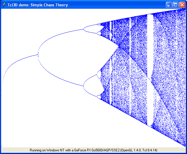

PO 2007/08/04

An enhanced version has been put onto a separate page Simple Chaos Theory with Tcl3D:

Implementation of slebetman's nice shading idea.
Interactive selection of chaos parameters.
Speed improvements by using a column cache.
Switch online between use of OpenGL or photo image for drawing.

slebetman Another variant, this time shaded - the more times a pixel is hit the darker it gets:

  # Implementation using image
  set width 640
  set height 480

  image create photo CANVAS -width $width -height $height

  pack [label .l -image CANVAS] -fill both -expand 1
  wm resizable . 0 0

  proc incrpixel {x y colorspec {reverse {}}} {
    foreach {RR GG BB} $colorspec break
    foreach {r g b} [CANVAS get $x $y] break
    set orig [color $r $g $b]
    
    foreach {c CC} {r RR g GG b BB} {
      set CC [set $CC]
      if {$reverse == "-reverse"} {
        set CC -$CC
      }
      set $c [expr {[set $c]-$CC}]
      if {[set $c] > 255} {set $c 255}
      if {[set $c] < 0} {set $c 0}
    }
    
    set CC [color $r $g $b]
    
    # don't need to waste CPU cycles if color doesn't change
    if {$CC != $orig} {
      CANVAS put $CC -to $x $y
    }
  }

  proc color {r g b} {
    return "#[format %02x $r][format %02x $g][format %02x $b]"
  }

  proc chaos {iterations colorspec {reverse {}}} {
    global width height
    
    set x .4
    
    if {$reverse == "-reverse"} {
      CANVAS put black -to 0 0 $width $height
    } else {
      CANVAS put white -to 0 0 $width $height
    }
    
    for {set sx 0} {$sx < $width} {incr sx} {
      set r_value [expr { pow(($sx*1.0)/$width, 0.25) * 3.0 + 1.0} ]

      for {set i 1} {$i <= $iterations} {incr i} {
        set x [expr {$r_value * $x * (1 - $x)}]
        # We're shading, no need to skip anything the starting
        # bits will simply be less dark if not near attractors.
        set sy [expr {int($height - $x*$height)}]
        incrpixel $sx $sy $colorspec $reverse
      }
      update
    }
  }
  
  chaos 800 {24 24 24}

  # uncomment the following to save image to file:
  #CANVAS write chaos.gif -format gif

You can also draw on a black canvas by specifying -reverse. And you can change colors by playing with the colorspec parameter. For example, this is red:

  chaos 800 {10 24 24}

and this is red on a black background:

  chaos 800 {24 10 10} -reverse

Increasing the colorspec values increases the overall brightness of the image. Increasing iteration increases the white point. Thus low colorspec numbers coupled with high number of iteration results in a high contrast image. Which leads to my favourite combination so far:

  chaos 2000 {8 10 14} -reverse

resulting in:

This next one took the better part of half an hour for me to render on my machine. But it nicely brings out patterns that I didn't notice before:

  chaos 6300 {3 3 3} -reverse

Category Mathematics

Category Plotting