Snippets Concepts Radioactive Decay
- Index for Snippets Concepts Radioactive Decay
- Limitations on Tool
- Extra Significant Figures, If Any in Debugging
- Introduction
- Body
- Key Steps
- Draft on Protocol
- Educational Applications
- Table 1 : Tcl Quality Guidelines
- Table. Use Extremely Descriptive, Honest Names (The #1 Rule)
- CVS Version of Table
- Table. Naming Variables, Code Quality Guidelines
- CVS Version of Table
- Appendix Code
- 1. Expanded Toy for Demo
- Output from ActiveState
- Output from Playground V9
- Toy Solver
- Page Is Under Development
- Hidden Comments Section
- Program Change Log
Index for Snippets Concepts Radioactive Decay
Preface
gold 2/9/2026. Here are some simple snippets for numerical methods. The goal is to use Tcl's minimalism as a learning tool. Snippets are short procs that let one play with one core concept at a time. All snippets are Playground V9 safe. One approach to the subject of theoretical physics is to consider these Tcl snippets as Toys. Some snippets here are listed as Toys. These Tcl procs are tiny entry points into physics. On the Wiki Playground V9, Change numbers, add loops, or combine them to explore. Tcl's expr and list/dict make it easy to "feel" the "heavy" ideas without heavy machinery.
Limitations on Tool
The TCL Snippets illustrate ideal mathematical behavior only and do not perform full simulation, actual measurements, or state vector evolution. The tool only visualizes ideal math structure, whereas no state vector simulation, probabilities, or actual measurement outcomes are derived. This tool for visualization does not simulate actual measurement outcomes or state vector evolution during operations. These are idealized protocols for tutorial purposes. Primarily, TCL /TK uses its strong points here for book keeping and displays. The example tool is not a full emulator. Meaning, limited scope for tutorial purposes.
Extra Significant Figures, If Any in Debugging
In debugging the calculations, some of the printout values reflect roughly 17-digit precision output from a typical double-precision computation. It's not "true exact" beyond 5 significant figures. Extra significant figures are used to check the calculations from other computer set-ups, not necessarily to infer accuracy of data measurements here. Typically, the slight differences in decimal places on far right of decimal point are normal floating-point behavior in Tcl's expr.
Advisor requests similar to previous snippets, but on topic of Radioactive Decay Model with Ruga-Kutta RK4 solution. I do not have all the answers. The Ideas Seemed to work, but maybe drawbacks?
Introduction
The page presents Tcl code snippets. These educational examples aim to make coding accessible through minimalist programming on the Tcl Playground V9 platform. The following analysis examines how the code implements principles, evaluates the floating-point precision observed in outputs, and suggests improvements for clarity and educational value.
Body
Key Steps
Draft on Protocol
gold This is a draft. 2/9/2026
The purpose of this article is to explain how a short Tool Control Language (Tcl) program simulates radioactive decay using a numerical method. The article will focus on two main ideas: the mathematical model for radioactive decay and the structure of the Tcl code that implements this model. The article will also explain how the program tests itself automatically so that a student or developer can check the result quickly.
Radioactive decay describes how a collection of unstable atomic nuclei loses members over time as the nuclei transform into other particles. The standard mathematical model states that the rate of change of the number of atoms is proportional to the number of atoms that remain. represents the initial number of atoms at time zero. The Tcl program does not solve this equation with an analytic formula but instead uses a numerical method that steps forward in time and approximates the solution.
The program begins by defining global parameters that describe the specific radioactive sample. The variable radioactiveDecayConstant stores the decay constant. The variable radioactiveDecayMaximumTime stores the final time for the simulation, and the variable radioactiveDecayNumberOfSteps stores how many equal time steps the program will use between the start and end of the simulation. A larger number of steps leads to smaller time step size and usually leads to a more accurate approximation of the exact solution, although the program will take longer to run.
The next key part of the program defines a general numerical integrator that uses the classical Runge–Kutta method of order four, often abbreviated as “RK4.” The Tcl procedure performOneFixedStepRungeKutta4 receives four inputs: the name of a derivative procedure, the current time, the current state vector, and the step size. The state vector is a list that can contain one or more components of the system; in this simple radioactive decay example, the state vector has only one component, which is the number of atoms. The step size is the amount of time that the integrator advances the solution in a single call. The RK4 method evaluates the derivative four times per step to provide a more accurate update than a simple Euler method.
Finally, the code combines the four derivative vectors with the standard RK4 weights 1,2,2,1 and scales the sum by one sixth of the step size to obtain the new state. This sequence allows a single procedure to advance any system of first order ordinary differential equations, not just the radioactive decay problem.
The program defines a derivative procedure that matches the physics of radioactive decay. The procedure calculateRadioactiveDecayRate receives the current time and a state vector. The procedure extracts the current number of atoms from the first element of the state vector. The procedure then computes the rate of change of the number of atoms as the product of the negative decay constant and the current number of atoms. The procedure returns this rate of change as a one-element list so that the performOneFixedStepRungeKutta4 procedure can treat it as a derivative vector. The time argument does not affect the derivative in this model, because the radioactive decay equation is autonomous. However, the argument remains present to keep the interface general and consistent with other models.
The main simulation procedure, runRadioactiveDecaySimulation, orchestrates the numerical experiment. The procedure builds the initial state vector as a one-element list that contains the initial number of atoms. The procedure sets the current time to zero. The procedure then computes the time step size as the maximum time divided by the number of steps. This computation ensures that the simulation finishes exactly at the designated maximum time. The procedure prepares two lists: listOfSimulationTimes and listOfNumberOfAtoms. At the beginning of the simulation, the procedure stores the initial time and initial number of atoms in these lists so that the lists contain a complete record from start to finish.
The loop inside runRadioactiveDecaySimulation carries out the integration. The loop runs from a step index of one up to the total number of steps. During each iteration, the procedure calls performOneFixedStepRungeKutta4 using the radioactive decay derivative procedure, the current time, the current state vector, and the time step size. The result becomes the new state vector for the next iteration. The procedure then increases the current time by one step. The procedure appends the new time and the new number of atoms to the storage lists. After the loop finishes, the lists contain the entire history of the simulation, including both time points and corresponding numbers of atoms.
The runRadioactiveDecaySimulation procedure returns the complete result as a Tcl dictionary. The dictionary contains four keys. The key times maps to the list of all time values used in the simulation. The key atoms maps to the list of numbers of atoms at each time point. The key t_final maps to the final time. The key state_final maps to the final state vector, which contains the final number of atoms. A user can inspect this dictionary from an interactive Tcl console, write the data to a file, or plot the data with an external tool.
The autotest procedure autotest_RadioactiveDecay supports quick checking of the code. The autotest procedure calls runRadioactiveDecaySimulation and stores the returned dictionary. The autotest procedure reads the final time and final state vector from the dictionary by using the dict get command. The procedure extracts the final number of atoms from the final state vector. The procedure prints the final time and the final value.
The autotest procedure then applies basic sanity checks that would catch obvious failures. The autotest procedure raises an error if the final time is less than or equal to zero, because a successful run should always advance time forward. The autotest procedure also raises an error if the final number of atoms is less than or equal to zero, because radioactive decay decreases the number of atoms but does not become negative in this simple model. The autotest procedure prints a success message if both checks pass.
The final line of the program calls autotest_RadioactiveDecay automatically when the file is sourced into the Tcl interpreter. This design turns the file into a self-testing module. A student can load the file into a Tcl session and immediately see whether the simulation behaves in a physically sensible way. A developer who modifies the code can rerun the same autotest to check that refactoring has not broken the model. For example, a developer might change the decay constant or increase the number of steps to improve accuracy, and the autotest procedure will still verify that the time increases and the number of atoms stays positive.
The program structure offers a useful pattern for other differential equation models. The Runge–Kutta integrator remains general and independent of the specific physics. A different model only needs a new derivative procedure that computes the rate of change for its own state vector. A population growth model, a cooling process, or a simple harmonic oscillator can all reuse the same performOneFixedStepRungeKutta4 procedure. The autotest concept can also carry over to other models by adjusting the reasonableness checks. For example, a population model autotest can check that the population does not become negative and that the total time matches the planned final time.
The program illustrates good practice in technical computing by combining a clear mathematical model, a reusable numerical core, explicit parameter definitions, and automatic testing. The descriptive variable names make the code easier to read than a version that uses single-letter names such as h or y. The clear separation between the integrator, the derivative function, and the simulation driver simplifies future modifications. A learner who studies this program can better understand both the physics of radioactive decay and the software structure that supports robust numerical experiments.
In conclusion, the Tcl program provides a compact but instructive example of numerical simulation of radioactive decay. The combination of a standard differential equation model, a reusable Runge–Kutta integrator, and a simple autotest routine creates a template that can be adapted to many other systems. A student or developer can use this pattern to build trustworthy numerical experiments that remain readable and maintainable over time.
Educational Applications
The program demonstrates math patterns.
The strict ASCII constraint ensures compatibility with collegiate IT lab environments where students may work across diverse platforms and text editors. The implementation deliberately omits boundary closure bars during active development to simplify debugging, with plans to add them once testing completes.
Table 1 : Tcl Quality Guidelines
| Priority | What good Tcl code usually has | What to avoid | Physics Relevance | Notes |
|---|---|---|---|---|
| 1 | Extremely clear names | x, tmp, data, temp1 | Momentum p → fourMomentum, z → celestialZ, ε → variationParameter | Clarity > brevity; physicists already spend cognitive load on concepts — don’t add more on variable names |
| 2 | Functions < 20–30 lines | 200-line monsters | One function ≈ one conceptual step (e.g. boost, projection, soft insertion) | Short procs mirror short proof steps — easier to verify correctness |
| 3 | One level of abstraction per function | Mix business + low-level details | Separate kinematics (4-vectors) from holographic map (z,\bar z) | Prevents mixing bulk physics with boundary CFT logic — aids conceptual separation |
| 4 | Consistent naming convention | camelCase + snake_case mix | Use snake_case for Tcl procs/vars (four_momentum, soft_factor) | Consistency reduces mental overhead when reading derivations or code |
| 5 | Meaningful distinction between similar concepts | user, usr, userData, theUser | Avoid p, pp, p_mu, pprime — prefer incoming_momentum, outgoing_momentum | In physics, small notation differences can hide big conceptual errors |
| 6 | Comments only when WHY is not obvious | Explaining WHAT good names already say | Comment the physical motivation (“# soft pole regulated for numerics”) | Most physicists read code like proofs — let names carry the story; comment intent |
| 7 | Domain language over technical language | processEntities → approveCustomerOrders | celestial_projection instead of map_to_sphere_coordinates | Use the language of celestial amplitudes, soft theorems, BMS group — makes code feel like theory |
Table. Use Extremely Descriptive, Honest Names (The #1 Rule)
Index number on draft is arbitrary.
| # | Bad / Cryptic | Good / Self-explaining | Why better? |
|---|---|---|---|
| 1 | x, tmp, data, i, res | userAgeInYears, temporaryPassword, allProducts | Immediately tells purpose |
| 2 | calc, process, doStuff | calculateTotalPriceWithTax, sendWelcomeEmail | Reveals what and why |
| 3 | getUser | findUserByEmail / getCurrentlyLoggedInUser | Different behaviors → different names |
| 4 | flag, status | isAccountActive, hasPaymentFailed, orderShipped | Boolean names should answer questions with yes/no |
| 5 | n, len, cnt | numberOfActiveUsers, totalItemsInCart | Avoid abbreviations unless universal (i→index ok) |
Note. Avoid one letter shortcuts on variable names.
CVS Version of Table
Index number on draft is arbitrary.
"#","Bad / Cryptic","Good / Self-explaining","Why better?"
"1","x, tmp, data, i, res","userAgeInYears, temporaryPassword, allProducts","Immediately tells purpose"
"2","calc, process, doStuff","calculateTotalPriceWithTax, sendWelcomeEmail","Reveals what and why"
"3","getUser","findUserByEmail / getCurrentlyLoggedInUser","Different behaviors → different names"
"4","flag, status","isAccountActive, hasPaymentFailed, orderShipped","Boolean names should answer questions with yes/no"
"5","n, len, cnt","numberOfActiveUsers, totalItemsInCart","Avoid abbreviations unless universal (i→index ok)"
Table. Naming Variables, Code Quality Guidelines
| Priority | What good code usually has | What to avoid |
|---|---|---|
| 1 | Extremely clear names | x, tmp, data, temp1 |
| 2 | Functions < 20–30 lines | 200-line monsters |
| 3 | One level of abstraction per function | Mix business + low-level details |
| 4 | Consistent naming convention | camelCase + snake_case mix |
| 5 | Meaningful distinction between similar concepts | user, usr, userData, theUser |
| 6 | Comments only when WHY is not obvious | Explaining WHAT good names already say |
| 7 | Domain language over technical language | processEntities → approveCustomerOrders |
Note. Avoid one letter shortcuts on variable names.
CVS Version of Table
"Priority","What good code usually has","What to avoid"
"1","Extremely clear names","x, tmp, data, temp1"
"2","Functions < 20–30 lines","200-line monsters"
"3","One level of abstraction per function","Mix business + low-level details"
"4","Consistent naming convention","camelCase + snake_case mix"
"5","Meaningful distinction between similar concepts","user, usr, userData, theUser"
"6","Comments only when WHY is not obvious","Explaining WHAT good names already say"
"7","Domain language over technical language","processEntities → approveCustomerOrders"
Screenshots Section
figure 1.
Snippets Concepts Radioactive Decay Playground Plot
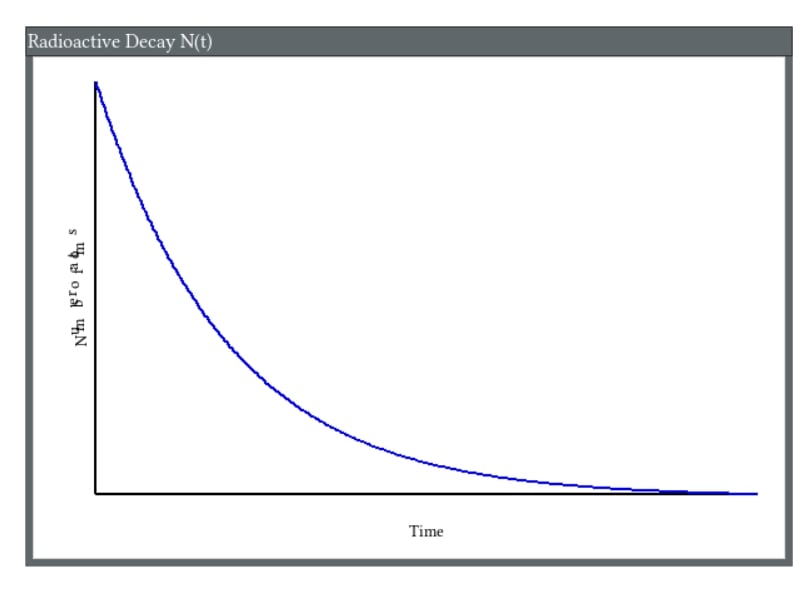
**** figure. RADIOACTIVE DECAY MODEL ****

+----------------------------------------------------------------------------------+
| RADIOACTIVE DECAY - Core Equation                                                |
|                                                                                  |
|    dN/dt = -λ × N                                                                |
|                                                                                  |
|    N(t)  = N₀ × e^(-λt)          (Analytical Solution)                          |
|                                                                                  |
|    λ     = decay constant                                                        |
|    N₀    = initial number of atoms                                               |
|    N(t)  = number of atoms remaining at time t                                   |
|                                                                                  |
|    Half-life = ln(2) / λ                                                         |
+----------------------------------------------------------------------------------+

**** figure. RUNGE-KUTTA RK4 INTEGRATION ****

+----------------------------------------------------------------------------------+
| RUNGE-KUTTA ORDER 4 (RK4) - Numerical Integration                                |
|                                                                                  |
|    k1 = f(t, y)                                                                  |
|    k2 = f(t + h/2, y + h·k1/2)                                                   |
|    k3 = f(t + h/2, y + h·k2/2)                                                   |
|    k4 = f(t + h,   y + h·k3)                                                     |
|                                                                                  |
|    y_new = y + (h/6)·(k1 + 2·k2 + 2·k3 + k4)                                    |
|                                                                                  |
|    Used in this snippet to solve dN/dt = -λN step-by-step                        |
+----------------------------------------------------------------------------------+

**** figure. RADIOACTIVE DECAY SIMULATION FLOW ****

+----------------------------------------------------------------------------------+
| RADIOACTIVE DECAY SIMULATION FLOW                                                |
|                                                                                  |
|    Set Parameters → λ, N₀, T_max, Steps                                          |
|             │                                                                    |
|             ▼                                                                    |
|    Initialize: t = 0, N = N₀                                                     |
|             │                                                                    |
|             ▼                                                                    |
|    Loop over steps:                                                              |
|        Compute k1, k2, k3, k4 using RK4                                          |
|        Update N(t)                                                               |
|        Store time and N(t)                                                       |
|             │                                                                    |
|             ▼                                                                    |
|    Output: List of times + atoms + Final N(t)                                    |
|    Run Autotest → Check final time > 0 and N(t) > 0                              |
+----------------------------------------------------------------------------------+

**** figure. ANALYTICAL vs NUMERICAL COMPARISON ****

+----------------------------------------------------------------------------------+
| ANALYTICAL vs NUMERICAL SOLUTION                                                 |
|                                                                                  |
|    Analytical (Exact)      N(t) = N₀ × e^(-λt)                                   |
|    Numerical (RK4)         Step-by-step approximation                            |
|                                                                                  |
|    Advantages of RK4:                                                            |
|      • Works for complex decay chains                                            |
|      • Easy to extend (add more variables)                                       |
|      • Good educational toy for understanding integration                        |
|                                                                                  |
|    Autotest verifies both time advances and N(t) stays positive                  |
+----------------------------------------------------------------------------------+

**** figure. EDUCATIONAL TOY STRUCTURE ****

+----------------------------------------------------------------------------------+
| EDUCATIONAL TOY - Radioactive Decay                                              |
|                                                                                  |
|    ┌─────────────────────┐                                                       |
|    │ Global Parameters   │  → λ, N₀, T_max, Steps                               |
|    └──────────┬──────────┘                                                       |
|               ▼                                                                  |
|    ┌─────────────────────┐                                                       |
|    │ RK4 Integrator      │  → performOneFixedStepRungeKutta4                     |
|    └──────────┬──────────┘                                                       |
|               ▼                                                                  |
|    ┌─────────────────────┐                                                       |
|    │ Decay Derivative    │  → dN/dt = -λN                                       |
|    └──────────┬──────────┘                                                       |
|               ▼                                                                  |
|    ┌─────────────────────┐                                                       |
|    │ Main Simulation     │  → runRadioactiveDecaySimulation                      |
|    └──────────┬──────────┘                                                       |
|               ▼                                                                  |
|          Autotest → Verify final results                                         |
+----------------------------------------------------------------------------------+

**** figure. LEFT-OVER CONCEPTS IN RADIOACTIVE DECAY ****

+----------------------------------------------------------------------------------+
| LEFT-OVER CONCEPTS IN RADIOACTIVE DECAY                                          |
|                                                                                  |
|    • Half-life remains meaningful even with numerical methods                    |
|    • Exponential decay appears naturally from linear differential equation       |
|    • Numerical methods (RK4) allow easy extension to coupled decay chains        |
|    • Autotest acts as a "sanity check" for physical realism                      |
|                                                                                  |
|    Educational value: Clear separation between model, integrator, and test       |
+----------------------------------------------------------------------------------+
References
- Snippets Physics Concepts Qubits
- Snippets Physics Concepts Feynman
- Snippets Physics Concepts Quantum
- Snippets Physics Concepts Toy
- Snippets Physics Concepts Minimalism
- Zero Handling Workarounds
Note. These Snippets on Theoretical Physics are a set, not stand alones. Recommend read all of the set.
Appendix Code
Appendix TCL Programs and Scripts
1. Expanded Toy for Demo
convert to strict 7-bit ASCII for Playground V9.
# may have to check strict ASCII for Playground V9
# Radioactive Decay Model V2
# Compatible with Tcl/Tk 8.6+
# TCL source code follows
# Written for Windows 11 on ActiveState Tcl
# Working on TCL Playground V9, strict ASCII only
# Optimized for collegiate IT lab environments
# Working under TCL version 8.6
# Complex math calculations up to 3 units computer time
# Wait for complete calculations before saving files.
# TCL club, 02/8/2026

# This is a hacker's patch, not rigorously derived.
# appears correct autotest
# pure ASCII code - no Unicode characters used anywhere
# omit next for Playground V9

#=====================================================================
# ''Radioactive Decay''
# dN/dt = -lambda * N
# Tcl 8.6+, pure ASCII, Playground V9 friendly
# =====================================================================

# omit next line for Playground V9
console show

# ---------------------------------------------------------------------
# Global configuration
# ---------------------------------------------------------------------

# Decay model parameters
set radioactiveDecayConstant                 0.1
set initialNumberOfAtoms                     1000.0
set radioactiveDecayMaximumTime              50.0
set radioactiveDecayNumberOfSteps            400

# =====================================================================
# Generic fixed-step RK4 integrator
# derivativeProcName currentTime stateVector -> derivativeVector
# stateVector is a Tcl list of state components
# =====================================================================

proc performOneFixedStepRungeKutta4 {derivativeProcName currentTime stateVector stepSize} {
    set stepSizeFull  $stepSize
    set stepSizeHalf  [expr {$stepSizeFull * 0.5}]

    # k1
    set derivativeVector_k1 [$derivativeProcName $currentTime $stateVector]

    # k2
    set temporaryStateVector {}
    foreach stateComponent $stateVector derivativeComponent $derivativeVector_k1 {
        lappend temporaryStateVector [expr {$stateComponent + $stepSizeHalf * $derivativeComponent}]
    }
    set derivativeVector_k2 \
        [$derivativeProcName [expr {$currentTime + $stepSizeHalf}] $temporaryStateVector]

    # k3
    set temporaryStateVector {}
    foreach stateComponent $stateVector derivativeComponent $derivativeVector_k2 {
        lappend temporaryStateVector [expr {$stateComponent + $stepSizeHalf * $derivativeComponent}]
    }
    set derivativeVector_k3 \
        [$derivativeProcName [expr {$currentTime + $stepSizeHalf}] $temporaryStateVector]

    # k4
    set temporaryStateVector {}
    foreach stateComponent $stateVector derivativeComponent $derivativeVector_k3 {
        lappend temporaryStateVector [expr {$stateComponent + $stepSizeFull * $derivativeComponent}]
    }
    set derivativeVector_k4 \
        [$derivativeProcName [expr {$currentTime + $stepSizeFull}] $temporaryStateVector]

    # Combine to get next state
    set nextStateVector {}
    foreach stateComponent $stateVector \
            k1Component $derivativeVector_k1 \
            k2Component $derivativeVector_k2 \
            k3Component $derivativeVector_k3 \
            k4Component $derivativeVector_k4 {
        lappend nextStateVector [expr {
            $stateComponent + $stepSizeFull
            * ($k1Component + 2.0*$k2Component + 2.0*$k3Component + $k4Component) / 6.0
        }]
    }
    return $nextStateVector
}

# =====================================================================
# Radioactive decay model: dN/dt = -lambda * N
# stateVector = {numberOfAtoms}
# =====================================================================

proc calculateRadioactiveDecayRate {currentTime stateVector} {
    set currentNumberOfAtoms [lindex $stateVector 0]
    set rateOfChangeNumberOfAtoms \
        [expr {-$::radioactiveDecayConstant * $currentNumberOfAtoms}]
    return [list $rateOfChangeNumberOfAtoms]
}

# ---------------------------------------------------------------------
# One full  run for radioactive decay
# Returns a dict for inspection / autotest:
#   times       -> list of times
#   atoms       -> list of N(t)
#   t_final     -> final time
#   state_final -> final state vector {N_final}
# ---------------------------------------------------------------------

proc runRadioactiveDecaySimulation {} {
    set currentStateVector     [list $::initialNumberOfAtoms]
    set currentTimeSeconds     0.0
    set timeStepSizeSeconds    [expr {$::radioactiveDecayMaximumTime \
                                      / double($::radioactiveDecayNumberOfSteps)}]

    set listOfSimulationTimes  [list $currentTimeSeconds]
    set listOfNumberOfAtoms    [list $::initialNumberOfAtoms]

    for {set integrationStepIndex 1} \
        {$integrationStepIndex <= $::radioactiveDecayNumberOfSteps} \
        {incr integrationStepIndex} {

        set currentStateVector [performOneFixedStepRungeKutta4 \
            calculateRadioactiveDecayRate \
            $currentTimeSeconds $currentStateVector $timeStepSizeSeconds]

        set currentTimeSeconds [expr {$currentTimeSeconds + $timeStepSizeSeconds}]

        lappend listOfSimulationTimes $currentTimeSeconds
        lappend listOfNumberOfAtoms   [lindex $currentStateVector 0]
    }

    return [dict create \
        times       $listOfSimulationTimes \
        atoms       $listOfNumberOfAtoms \
        t_final     $currentTimeSeconds \
        state_final $currentStateVector]
}

# =====================================================================
# Autotest block (runs radioactive decay dek when file is sourced)
# =====================================================================

proc autotest_RadioactiveDecay {} {
    puts "Running radioactive decay autotest..."

    set simulationResult        [runRadioactiveDecaySimulation]
    set finalTimeSeconds        [dict get $simulationResult t_final]
    set finalStateVector        [dict get $simulationResult state_final]
    set finalNumberOfAtoms      [lindex $finalStateVector 0]

    puts [format "Final time:       %.3f"  $finalTimeSeconds]
    puts [format "Final N(t):       %.6f"  $finalNumberOfAtoms]

    if {$finalTimeSeconds <= 0.0} {
        error "Autotest failed: radioactive decay final time is non‑positive"
    }
    if {$finalNumberOfAtoms <= 0.0} {
        error "Autotest failed: radioactive decay number of atoms went non‑positive"
    }

    puts "Radioactive decay autotest passed."
}

# Run autotest automatically when this file is sourced.
autotest_RadioactiveDecay
Output from ActiveState
Running
Autotest passed.
(bin) 1 %
VolterrRunning radioactive decay autotest...
Final time:       50.000
Final N(t):       6.737947
Radioactive decay autotest passed.
Output from Playground V9
> }
(tcl) 35 %
(tcl) 55 %
(tcl) 55 % # Run autotest automatically when this file is sourced.
(tcl) 56 % autotest_RadioactiveDecay
Running radioactive decay autotest...
Final time:       50.000
Final N(t):       6.737947
Radioactive decay autotest passed.
(tcl) 57 %
Toy Solver
Page Is Under Development
This page is under development. Comments are welcome, but please load any comments in the comments section at the bottom of the page. Please include your wiki MONIKER and date in your comment with the same courtesy that I will give you. Aside from your courtesy, your wiki MONIKER and date as a signature and minimal good faith of any internet post are the rules of this TCL-WIKI. Its very hard to reply reasonably without some background of the correspondent on his WIKI bio page. Thanks, gold 5Jan2026
gold 2/9/2026. Added categories, so can find message in Wiki.
Hidden Comments Section
Program Change Log
gold 2/3/2025. Testing, encountered initial difficulty in saving work? Long code blocks with or unmatched wiki markup can sometimes confuse the Tcl Wiki formatting engine, especially if fences are not balanced or a line begins with markup it treats specially.
gold 2/4/2025. Added Automatic Dump of Examples, Using ActiveState. Added temp double hatch border, ##.
Please place any comments here with your wiki MONIKER and date, Thanks.gold 1/30/2026
Note. Testing computer methods and computer programs, maybe wrong numbers.
| Category Numerical Analysis | Category Toys | Category Calculator | Category Mathematics | Category Example | Toys and Games | Category Games | Category Application | Category GUI |