Snippets Concepts Classical Oracle Simulation for Grover Search
- Index for Snippets Concepts Classical Oracle Simulation for Grover Search
- Preface
- Limitations on Tool and Disclaimer
- Extra Significant Figures, If Any in Debugging
- Introduction
- Important Disclaimer About Expectations
- Classical Simulation versus Quantum Simulation
- What if My Boat Becomes an Electron with Electron Wake, Still too Big for Quantum Effects?
- Potential Uses for This Classical Oracle Function in Tcl or Python, Non-Quantum
- Scalable Limits to Oracle Implementation in Classical Proc
- Would ASCII diagrams be suitable for Displaying a Quantum Solution?
- Summary
- Wiki Table: Grover's Algorithm Timeline
- Wiki Table: Logical Qubit Milestones and Benchmarks Timeline
- Wiki Table: Shor's Algorithm Timeline – Key Milestones
- References
- Testing Extended deck,
- Result in Wiki Tables from Active State
- Grover Wiki Table Report
- Wiki table for Auto Test 1 (Max State 7, Iterations 2)
- Wiki table for Auto Test 2 (Max State 7, Iterations 2)
- Wiki table for Auto Test 4 (Max State 15, Iterations 3)
- Wiki table for Auto Test 5 (Max State 15, Iterations 2)
- Draft Figures, ASCII Diagrams for Simulation program flow
- Important Caution on ASCII Diagrams
- Flow Diagrams for the Classical TCL Programs, following
- Figure. Tcl Oracle Module Program Flow
- Draft. ASCII Diagrams for the Projected Python-Qiskit Solution, following
- Draft. Circuit ASCII Diagrams
- Draft Figure. 2 Qubit Grover Circuit, Marked State 1
- Draft Figure. 3 Qubit Grover Circuit, Marked State 7
- Draft Figure. 2 Qubit Grover Circuit, Marked State 2 (Centered)
- Draft Figure. 3 Qubit Grover Circuit, Marked State 4 (Centered)
- Figure. Standard Diffuser Block
- Figure. GRAPH 1 – INITIAL UNIFORM DISTRIBUTION
- Figure. GRAPH 2 – AFTER ORACLE (Phase Flip on Winning State)
- Figure. GRAPH 3 – AFTER FIRST DIFFUSION (Reflection About Mean)
- Figure. GRAPH 4 – 2-QUBIT GROVER CIRCUIT (Marked State 01)
- Algorithm Circuit Glossary for Wiki Page, Draft
- Hidden Comments Section
- Program Change Log
- Draft Figure. 2 Qubit Grover Circuit, Marked State 1
- Draft Figure. 3 Qubit Grover Circuit, Marked State 7
- Draft Figure. 2 Qubit Grover Circuit, Marked State 2 (Centered)
- Draft Figure. 3 Qubit Grover Circuit, Marked State 4 (Centered)
Index for Snippets Concepts Classical Oracle Simulation for Grover Search
Preface
gold 7/22/2026. Advisor and discussion has requested snippets on Classical Oracle Simulation, notably as used in the Grover's Search Algorithm. The simulation model is intended as an exploratory or experimental framework for TCL/TK coding. The full up algorithm is normally run on Quantum computers using Quantum feasible languages. Task Statement: generate a tutorial simulation of algorithm for a classical computer in pure TCL 8.6+. Adding references to Dr. Chiara Marletto's counterfactual framework from the book "The Science of Can and Can't" along with other perspectives. We are using modular snippets inside modular structured programs. Page content is targeted for engineering students and other Quantum tutorials.
gold 7/22/2026. Upon review of draft page, First Advisor .... what about the difference between TCL/TK [ classical algorithms ] and the [ proposed ] quantum implementations?
I do not have all the answers. The Ideas Seemed to work, but maybe drawbacks? When measured by the Tcl timing statements, completion times and solutions of parameters will differ on different computer set-ups. Assume a future maintainer, either AI Model or human programmer, would have to maintain code with info content and explanatory variable name in program, ref "Snippets Concepts Effects". The Nassi Shneiderman Diagrams NSD or pseudocode Flowcharts pertain to the Tool Control Language TCL computer language as well as other computer languages like Python 3, pseudocode, word logic problems, and technical reports.
For each logic condition selecting a path or calculation task, we might have one, two, or multiple deterministic branches. Attempting to adapt format to multiple probabilistic branches used in Artificial Intelligence AI Models. Then we may use the >>> lottery algorithm <<< to select the winning pathways or tickets.
The existing program has some dummy subroutines. A full construction seems too complex here. I found a paper with images of quantum walks, and I’m wondering if it’s possible to simulate the curves shown in the charts. My advisor has suggested that quantum entanglement/superposition could simulate or underlie quantum worlds, but I’m not sure that I agree. I have limited space on the wiki page, and the fill‑in for the dummy routines has to be pretty brief. In engineering terms, I’m aiming for a “90% solution”, meaning about 90% right and 10% off. Like the simple college formula for a pendulum that is not the exact time series. Call it “prototype it ’til you make it” as a college try, but for Quantum Many Worlds. Who is to say? Perhaps you know, TcL specializes in GUI solutions. Maybe try and adapt some starter TcL code for a "quantum worlds slide rule ". Hopefully compatible with the hard-wired classical theory.
Limitations on Tool and Disclaimer
The TCL Snippets illustrate ideal mathematical behavior only and do not perform full simulation, actual measurements, or state vector evolution. The tool only visualizes ideal math structure, whereas no state vector simulation, probabilities, or actual measurement outcomes are derived. This tool for visualization does not simulate actual measurement outcomes or state vector evolution during operations. These are idealized protocols for tutorial purposes. Primarily, TCL /TK uses its strong points here for book keeping and displays. The example tool is not a full emulator. Meaning, limited scope for tutorial purposes.
Disclaimer. None of the computer programs, numerical experiments, power-law fits, or physical analogies described here give a strict, formal proof of the Conjectures, either individually or in combination. The tools and analogies are heuristic models and visualization tools that follow engineering “rules of thumb.” Whereas, pure mathematics has its own shop rules for what counts as a rigorous proof. Any opinions on the difficulty or plausibility reflect current understanding here and programming of the Conjectures as a very hard open problem, not a completed exact math proof, and are offered with full respect for the standards of professional mathematicians.
Extra Significant Figures, If Any in Debugging
In debugging the calculations, some of the printout values reflect roughly 17-digit precision output from a typical double-precision computation. It's not "true exact" beyond 5 significant figures. Extra significant figures are used to check the calculations from other computer set-ups, not necessarily to infer accuracy of data measurements here. Typically, the slight differences in decimal places on far right of decimal point are normal floating-point behavior in Tcl's expr.
Introduction
gold 7/22/2026. A classical Oracle Black Box Simulation. It uses Grovers search as an example, but everything stays classical. In this case the Oracle function ends up being a regular TCL procedure. That means it runs like any other TCL function without needing quantum hardware. The "Oracle" used here is a standard classical procedure, not a quantum routine. Real quantum algorithms using oracles can offer theoretical speedup on actual quantum hardware, but this classical simulation does not provide any quantum advantage. It is intended only for learning and conceptual understanding. Please do not expect this code to run faster than any other classical search methods on large problems. The code is a teaching tool, not a practical quantum computer.
Real hardware has noise, error correction overhead, and implementation costs. These Toy Models are idealized for tutorial purposes, not final engineering estimates.
Important Disclaimer About Expectations
- This code is a classical simulation of an algorithm.
- It runs entirely on a normal classical computer using Tcl/Tk.
- It does not provide quantum speedup.
- It is for educational and conceptual understanding only.
- Real quantum computers (when large enough) may offer quadratic speedup for search problems
- Quantum Speedup requires actual quantum hardware and error correction.
- The Oracle concept by itself is not quantum only.
- The Oracle concept is a classical black-box function used within quantum feasible languages.
Clarifying the "Oracle" Concept. Many people become confused when they hear the word Oracle in quantum computing. Many assume that the Oracle is a purely quantum routine that only runs on a real quantum computer. In Qiskit and most quantum SDKs, the Oracle is almost always a classical function written in Python. Meaning, Python that runs on a normal classical computer.
Details. Python-Qiskit code runs on classical hardware unless a quantum backend is explicitly used. Oracle like subcircuits can appear in both Grover and Shor Algorithms. But typically, Grover uses an obvious and so-named Oracle Function. Some later implementations of Shor and other Quantum Algorithms may hide that same idea and similar functions inside other Quantum circuit components, and maybe unnamed in the code.
Classical Simulation versus Quantum Simulation
Draft. The selected algorithms are very different in classical languages like TCL/TK and Python versus Quantum computer algorithms in Python-Qiskit. Classical simulation runs on a normal computer. Classical methods use ordinary math and loops. Classical does not touch real qubits, by definition here. Classical computers do not provide quantum speedup.
Draft. There are shades of meaning here. Quantum computer algorithms in Python-Qiskit build real quantum circuits of qubits. Python-Qiskit uses qubits and gates to create a true quantum state (eventual solution). Quantum computer algorithms may run through either a Quantum simulator or a Quantum hardware backend to produce quantum results. That Quantum simulator in Python-Qiskit is still classical until the Quantum hardware fired up. In other words, the Quantum simulator ref Python-Qiskit does not give Quantum Speedup. Only the Quantum hardware gives Quantum Speedup. Refer to the IBM Quantum Platform, Python-Qiskit Quick Start. Also, the textbook "Learn Quantum Computing using Qiskit' on Github.
What if My Boat Becomes an Electron with Electron Wake, Still too Big for Quantum Effects?
This is analogy and preparation for Coding, with some humor.
Those wakes you are seeing behind the speedboat is classical wave phenomenon. Water waves are collective behavior of water molecules on disturbance. While waves in water do show the wave like properties of interference, reflection, and diffraction. On the human scale, those wakes and water waves are not exhibiting quantum or wave-particle duality in any human observable way.
But on the Quantum scale, there is a wonderful surprise in nature. “Boat becomes an electron” may be equivalent analogy to radiation track physics, RTP. Because radiation track physics is an example where quantum effects do produce visible wave like structures in matter.
Nature makes a rare event observable in RTP by amplifying the Quantum effects along a path. Grover’s Algorithm does something similar in Quantum information space. Grover’s Algorithm amplifies the “signal” for the item search. Hopefully, the search signal stands out clearly against the background field, like a powerful search light. Opps, mixing Quantum analogies here.
Watch dial electrons fall to their ground state. Electrons release energy as visible light You almost have Me convinced, but would diffusion or spread of alpha path be a quantum effect, ref Einstein? Meaning, granted the Alpha/Beta diffusion path is normally modeled as Einstein-style random walk, even though the underlying collisions are Quantum Mechanical. Not to do a Sales job, but would the Grover software model the possible Quantum Diffusion or not? You see, you and I have created the Grover software model that is looking for a cushy job like yours. Joke.
Suppose I spun up the Groover axis like a Tibetan prayer wheel, would that simulate diffusion enough to get Grover software hired on. If you don't like constant rotation rate, how about multiple eccentric gears or slip clutch systems? A few extra eccentric gears, and no human would recognize the pattern easily. Maybe the chief electric detective might. Light diode indicators and “amplitude tell tales” that pop off when the marked Groover states are dialed in or alignment achieved on the mystic wheel.
Potential Uses for This Classical Oracle Function in Tcl or Python, Non-Quantum
Here are practical examples for the same Oracle Function in various classical computer tasks. Pattern & Search / Filtering Tool would find records in a database or list that match certain criteria. A Constraint Solver would be Sudoku, N-Queens, or scheduling problems. Also, include mark valid configurations. Optimization Problems might include Traveling Salesman, Knapsack, or resource allocation. Pattern Matching might be search for specific patterns in strings, numbers, or game states. Educational Tools might be teaching classical search algorithms, backtracking, or brute-force versus smarter methods. Game AI artificial intelligence would be to mark winning board positions in Tic-Tac-Toe, Chess endgames, etc.
Scalable Limits to Oracle Implementation in Classical Proc
Scaling in code refers to metrics as program keeps working as the input size, number of users, or amount of parameters/data grows.
There is one limiting structural difference between the Tcl syntax and design of practical quantum circuits. A Tcl list works with any length, so the original Proc version took any $max_state. Quantum registers only allow sizes that are powers of two. This means the $max_state has to be one less than a power of two such as 7 15 or 31. This is effectively a constraint on the practical number of Qubits in the solution circuit. By inspection, the original autotests were limited to circuits of 1,2,3,4,5 qubits. The first case of 1 Qubit circuit was an edge or corner testcase, no solution seen.
For the Oracle simulation in Tcl, the Number of Qubits in the Quantum circuit has to be capped because of lengthy laptop computation times beyond 10 qubits. Comfortable use on a Windows 11 laptop might be about 5 to 6 qubits at 32 to 64 states. A normal laptop becomes painfully slow around 10–12 qubits at 1,024 to 4,096 states. The Tcl Oracle simulation is assessed impractical beyond 15 qubits at 32,768+ states.
eval { 2**N } is formula
eval { 2**5 }  = 32
eval { 2**6 }  = 64
eval { 2**10 } = 1024
eval { 2**12 } = 4096
eval { 2**15 } = 32768
All the existing autotest cases already fit these constraints on $max_state and N, so practice did not change at all. A new test case would need to follow that constraint.
Would ASCII diagrams be suitable for Displaying a Quantum Solution?
Draft. Concerning the projected solution in the proposed Python-Qiskit Port, would ASCII diagrams be suitable? The main flow might be shown in ASCII diagrams, I suppose, but would parallel, phased, timing, or simultaneous channels be adequately shown, without some understood notation changes? If there is a perceptible quantum circuit designed in Python-Qiskit, I would be interested in the 2‑ and 3‑qubit circuits.
Summary
Typically, Classical computers need many more trials and much computer time to gain extra decimal places of accuracy. The TCL/TK coding can be used to model or simulate those portions or stages of a Quantum Algorithm that may use a classical computer. These are Toy Models and simplified estimates for tutorial purposes.
Classical Oracle simulation offers a clear way to understand how search behaves without using a quantum device. The Classical simulation helps beginners and students see how the search pattern emerges from repeated queries. The same ideas and ideas prepare students for later work with real quantum circuits. That is, when stable hardware becomes available.
Wiki Table: Grover's Algorithm Timeline
Lov Grover developed Grover's algorithm in 1996. The algorithm provides a quadratic speedup for unstructured search problems. Grover's work complements Shor's algorithm and serves as a core primitive in many quantum algorithms.
Wiki Table: Grover's Algorithm Timeline – Key Milestones
| Index | Year | Event | Note |
|---|---|---|---|
| 1 | 1996 | Lov Grover proposes the algorithm | Indian-American computer scientist at Bell Labs introduces quantum search with quadratic speedup |
| 2 | Late 1990s | Theoretical extensions | Researchers develop amplitude amplification framework and applications beyond search |
| 3 | Early 2000s | First experimental demonstrations | Teams implement small-scale versions using nuclear magnetic resonance and other platforms |
| 4 | 2000s–2010s | Photonic and ion trap implementations | Groups demonstrate Grover search on photonic qubits and trapped-ion systems |
| 5 | 2010s | Superconducting qubit experiments | Research teams run Grover's algorithm on superconducting processors with increasing qubit counts |
| 6 | 2020s | Scalable and optimized implementations | Teams focus on noisy intermediate-scale quantum devices, error mitigation, and larger search spaces |
| 7 | 2020s | Applications in state preparation and optimization | Researchers adapt Grover techniques for quantum machine learning and combinatorial problems |
| — | Ongoing | Hardware and hybrid efforts | Multiple groups pursue fault-tolerant versions, classical simulations, and integration with other quantum algorithms |
Wiki Table: Logical Qubit Milestones and Benchmarks Timeline
| Index | Year | Event | Note |
|---|---|---|---|
| 1 | 2010s | Early small-code experiments | Teams demonstrate basic error detection on few-qubit repetition and stabilizer codes |
| 2 | 2019–2022 | Google Quantum AI surface code scaling | Demonstrates error reduction by increasing physical qubits in surface code logical qubit |
| 3 | 2023–2024 | Beyond break-even demonstrations | Google achieves logical error rate below physical qubit rate with surface code |
| 4 | 2024 | IBM quantum low-density parity check codes | IBM demonstrates [144,12,12] bivariate bicycle code encoding multiple logical qubits |
| 5 | 2024–2025 | Neutral atom and trapped-ion advances | Companies like QuEra, Quantinuum, and Atom Computing report logical qubit experiments with competitive overhead |
| 6 | 2025–2026 | Industry benchmarking frameworks | Alice & Bob and others propose standardized five-criteria evaluation for logical qubit claims |
| 7 | 2020s | Multi-logical-qubit operations | Teams progress toward logical gates and small algorithms on encoded qubits |
| — | Ongoing | Scaling and standardization | Research focuses on distance scaling, real-time decoding, and magic state distillation benchmarks |
Wiki Table: Shor's Algorithm Timeline – Key Milestones
Peter Shor's work sparked intense interest in quantum computing as a practical technology.
| Index | Year | Event | Note |
|---|---|---|---|
| 1 | 1994 | Peter Shor proposes the algorithm | American mathematician at Bell Labs introduces polynomial-time quantum factoring and discrete logarithm solution at the Foundations of Computer Science conference |
| 2 | 1994–1995 | Initial theoretical refinements | Researchers analyze circuit complexity and error correction needs for fault-tolerant execution |
| 3 | 2001 | First experimental demonstration by IBM team | IBM Research-Almaden group factors 15 using 7-qubit liquid-state nuclear magnetic resonance quantum computer |
| 4 | Early 2010s | Photonic and solid-state implementations | Independent teams demonstrate variants; one photonic setup factors 21 |
| 5 | 2012 | Superconducting processor demonstration | Team achieves factorization of 15 on superconducting qubits |
| 6 | 2016 | Trapped-ion implementation | Researchers factor 15 with trapped-ion qubits and qubit recycling technique |
| 7 | 2019 | Larger number attempt on IBM Q System One | Team attempts to factor 35 on superconducting hardware |
| 8 | 2020s | Resource estimation and compilation focus | Multiple teams optimize circuits, reduce qubit and gate counts, and address noise limitations |
| — | Ongoing | Hardware and simulation efforts | Research groups worldwide pursue scalable versions, error-corrected demonstrations, and educational tools |
References
- Snippets Concepts DFT on Inference Vectors
- Snippets Concepts Triangular Propagation
- Snippets Concepts Inference Engine
- Snippets Concepts Diósi Penrose Model
- Snippets Concepts Quantum Fourier Transform
- Snippets Concepts Lottery Pruning
- Snippets Concepts Qubits Model
- Snippets Concepts Collatz Plotter
- Snippets Concepts Geometric Tunneling
- Snippets Concepts Collatz T-Stop
- Snippets Concepts Random Cubics
- Snippets Concepts McCarthy 91_Function
- Snippets Concepts Predator Prey
- Snippets Concepts Thomas Solver
- Snippets Concepts Grover Simulation
- Snippets Concepts Radioactive Decay
- Snippets Concepts Hypersphere Simulation
- Snippets Concepts Nassi Shneiderman Flowcharts
- Snippets Concepts SlideRule to Quantum
- Snippets Physics Concepts Qubits
- Snippets Physics Concepts Feynman
- Snippets Physics Concepts Quantum
- Snippets Physics Concepts Toy
- Snippets Physics Concepts Minimalism
- Zero Handling Workarounds
Note. These Snippets on Theoretical Physics are a set, not stand alones. Recommend read all of the set.
- A little slide-rule on TCL Wiki, ( much credit for the algorithms in the sliderule. )
- Richard Suchenwirth 2003-08-31
- Smoothing and differentiation of data by simplified least squares procedures
- Savitzky, A. ; Golay, M. J. E. Two examples are presented as subroutines in the FORTRAN language.
- Savitzky Golay Filtering, Python
- Savitzky Golay Filtering — SciPy Cookbook documentation
- Smoothing Example with Savitzky-Golay Filter in Python
- Introduction to the Savitzky-Golay Filter: A Comprehensive Guide (Using Python), Thomas Konstantinovsky
- Konstantinovsky has good explanation. Note detailed. WhittakerSmoother in Python
- The Perfect Way to Smooth Your Noisy Data, Whittaker-Eilers smoother, Andrew Bowell
- Feb 28, 2024
- A Basis for a Mathematical Theory of Computation,Author(s)
- McCarthy, John
- John McCarthy: A basis for a mathematical theory of computation, in:
- Computer Programming and Formal Systems.
- P.Braffort, D.Hirschberg (ed.), Amsterdam:North Holland 1963,
- several versions, archived pdf
- McCarthy’s LISP and Basis for Theory of Computation, archived pdf
- en.wikipedia.org search on <John McCarthy computer>
- John McCarthy at Stanford web site, archived
- Towards a Mathematical Science of Computation, J. McCarthy,
- Computer Science Department, Stanford University, archived pdf
- Elephant 2000: A Programming Language Based on Speech Acts
- John McCarthy, Stanford University, archived
- Elephant input and output statements are characterized
- as speech acts and programs, which
- can refer directly to the past.
- Elephant proposal contains summary
- on McCarthy mathematical theory of computation
- Mysteries and other Matters, development of Lisp , archived
- Note. A lot of early papers and notes from John McCarthy and Knuth are difficult to assess web links or archived.
- Machine Learning Approaches to the Collatz Conjecture:
- A Comprehensive Framework for Pattern Recognition
- and Automated Conjecture Generation. IJIRT, Vol. 12 Issue 7
- Transformers Know More Than They Can Tell:
- Learning the Collatz Sequence , arXiv:2511.10811
- The Collatz conjecture, Littlewood-Offord theory, and powers of 2 and 3,
- Aug 2011, Terence Tao,
- mentions Gambler's Ruin on this 2011 post, but better search on his website for updates.
- Efficient Computation of Collatz Sequence
- Stopping Times: A Novel Algorithmic Approach ( credit for the new algorithm. )
- EYOB SOLOMON GETACHEW, BEAKAL GIZACHEW ASSEFA
- The Collatz Conjecture over the Gaussian Integers, Alejandra Alvarado
- An example of the difference between quantum and classical random walks
- Andrew M. Childs, Edward Farhi, Sam Gutmann ( much credit for the new algorithm. )
- Simple Program Design, Lesley Anne Robertson, 2004
- Lecture in Spanish, diagrama de nassi schneiderman o rectángular
- website for estudia con nancho, 2023
- Lecture, Communicating Complex Logic with Ease
- with Nassi-Shneiderman Diagrams, Atanas Marchev,
- Jetbrains MPS community, 2023
- Java library for working with Nassi-Shneiderman diagrams
- (structograms) from Atanas Marchev, Github website
- Flowchart techniques for structured programming
- Authors: I. Nassi, B. Shneiderman, circa 1973
- KernelF- an Embeddable and
- Extensible Functional Language, Markus Voelter
- voelter = acm, ~~ 2023
- Algorithmic Accountability: Designing for Safety , Ben Shneiderman,
- Radcliffe Institute, 2018
- the lottery ticket hypothesis:
- finding sparse, trainable neural networks, jonathan frankle, mit
- 4 mar 2019, michael carbin
- Maria Violaris, arXiv preprint titled "Quantum observers can communicate across multiverse branches." Jan 2026
- Vafa, Cumrun (September 2006). "Baby universes and string theory". International Journal of Modern Physics D. 15 (10): 1581–1586.
- Lecture from Sean Carroll: The many worlds of quantum mechanics
- Lecture from Sean Carroll: Quantum Mechanics and the Many-Worlds Interpretation
- Lecture on many worlds theory, Does Quantum Mechanics Reveal the Secrets of Parallel Universes?
- Emergence of Classicality in Wigner’s Friend Scenarios, Tom Rivlin, Jul 2025
- Quantum Superpositions of Conscious States in a Minimal Integrated Information Model, Kelvin J. McQueen, April 2026
- Wigner's friend scenarios: on what to condition and how to verify the predictions
- Flavio Del Santo, Jul 2024
- A review and analysis of six extended Wigner's friend arguments
- David Schmid, Yìlè Yīng, Matthew Leifer, Aug 2023
- The Many Worlds of Hugh Everett III : Multiple Universes,
- Mutual Assured Destruction, and the Meltdown of a Nuclear Family
- Peter Byrne, 2010
- The Many-Worlds Interpretation of Quantum Mechanics (level 3 multiverse), dissertation,
- Everett, Hugh
- An Undergraduate Course in Quantum Computing, Peter Young, Apr 2026
- # Based on ref. An Undergraduate Course in Quantum Computing, Peter Young, Apr 2026
- # Much credit for the quantum circuit diagrams, Matches textbook Fig 16.4 etc
- # University of California Santa Cruz, CA, arXiv:2604.10396
- Does gravity follow the rules of quantum mechanics? Press Release, Prof. Kazuhiro Yamamoto
- Momentum squeezed state realized via optimal filtering in optomechanics:
- Implications for gravity-induced entanglement”, Ryotaro Fukuzumi, Published 13 April,2026.
- Bose-Marletto-Vedral experiment without observable spacetime superpositions
- Nicetu Tibau Vidal,Chiara Marletto
- The Science of Can and Can't : A Physicist's Journey Through the Land of Counterfactuals
- by Chiara Marletto, 2021.
- Quantum Coins and Counterfactuals, in Consistent Quantum Theory, Robert B. Griffiths, 2002,
- from CMU Quantum Theory Group
- How to Rewrite the Laws of Physics in the Language of Impossibility,
- Amanda Gefter, Contributing Writer, April 29, 2021
- Fundamental properties of beam-splitters in classical and quantum optics: arxiv /abs/2303.13705
- Masud Mansuripur, Ewan M. Wright, 2023
- Constructor theory, Wikipedia, date 4/27/2026
- Constructor theory of probability, 2016,
- Chiara Marletto
- Bernstein, G. A. (2026c). Reality is mathematical structure.
- Bernstein, G. A. (2026e). Why these simple laws?
- Deriving physics from mathematical necessity.
- Bernstein, G. A. (2026h). The arrow of time is irreversible computation.
- Deutsch, D. (2013). Constructor theory. Synthese, 190(18), 4331-4359.
- Deutsch, D., & Marletto, C. (2015). Constructor theory of information. Proceedings of the Royal
- Society A, 471(2174), 20140540.
- Deutsch, D. (1997). The Fabric of Reality. Penguin.
- Deutsch, D. (2011). The Beginning of Infinity. Penguin.
- Marletto, C. (2021). The Science of Can and Can't. Penguin.
- Popper, K. (1972). Objective Knowledge. Oxford University Press.
- The Shor’s Algorithm is public domain,
- and mathematical knowledge since 1994.
- Peter Shore, Original 1994 Conference Paper
- Algorithms for Quantum Computation: Discrete Logarithms and Factoring
- Peter Shore, Polynomial-Time Algorithms for Prime Factorization
- and Discrete Logarithms on a Quantum Computer (1995 expanded version)
- IBM Quantum Platform, Python-Qiskit Quick Start, 2020
- Also, the textbook "Learn Quantum Computing using Qiskit' on Github,
- Credit. Rafey Iqbal Rahman, 2020
TCL Wiki has numerous excellent pages on Monte Carlo methods, largely from arjen .
- A simple Monte Carlo simulation,
- Evaluation of multiple integrals using quasi-random points,
- Markov chain Monte Carlo
- Poisson distribution
Note. The ink is hardly dry on some of these papers. Don't know what gems are hidden, if I dig deeper.
Screenshots
Figure. Classical GUI Mockup
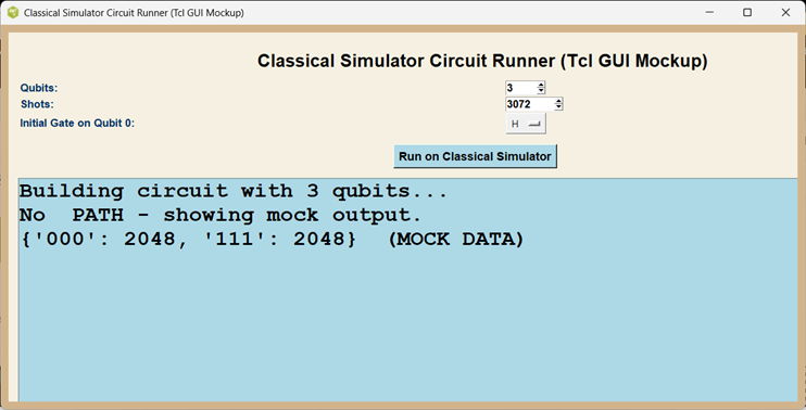
Figure. Coding Analogy of Grover's Speedboat

Figure. Coding Analogy of Grover's Speedboat, 1.1 MB

Testing Extended deck,
Due to the space on wiki page, I am omitting some wordy explanatory comments inside the deck, while debugging. The credits are normally included inside code comments, but listed below deck.
# Classical Simulation of Oracle Function Algorithm  V5
# in pure Tcl 8.6+ for tutorial purposes.
# Tcl 8.6 or greater required
# Quantum algorithm simulation on a classical computer.
# Classical Simulation code does not provide Quantum Speedup.
# Quantum Speedup requires actual Quantum hardware,
# Quantum feasible algorithms, and Quantum Error Correction QEC.
# Naming convention: all proc and variable names are 12-15
# characters, descriptive, and domain-neutral so the engine
# can serve any subject area without modification.
#
# ----
# Compatible with Tcl/Tk (Tool Command Language / Toolkit) 8.6+
# Written for Windows 11 on ActiveState Tcl.
# Use Pure 7-bit ASCII code, no Unicode characters used anywhere.
# ----
# Using modular snippets inside modular structured programs.
# Modules should be 15 to 25 lines long without comments.
# Small length modules
# are believed to aid future  code maintenance.
# Program deck may contain multiple estimation procs.
# Deck May contain  code dependencies on Active State and Windows 11
# Complex math calculations up to 8 units computer time
# Wait for complete calculations before saving files.
# Proc names and variables names need to be very human readable
# and very explanatory.
# Avoid variables with single letter names.
# Whereas single letter names are known to lead
# to many historic errors.
# Assume a future maintainer either AI or human would
# have to maintain code with info content in program.
# This is Experimenting Draft Prototype,
# and not a replacement for TCL Core.
# This is a prototype's patch, not rigorously derived.
# appears correct solutions for autotests.
# The Grover Oracle is listed as a namespace.
# This is a prototype's patch, not rigorously derived.
# appears correct solutions for autotests.
#
# File contains the revised oracle module.
# This file will be base of the QAE algorithm.
# TCL Club 8/5/2026
#
if {[llength [info commands console]] > 0} {
    console show
}

namespace eval ::grover_engine {

# oracle module: pure oracle state; default list empty
    namespace eval oracle {
        namespace path [list ::grover_engine]
        variable good_solutions {}

        proc set_solutions {new_list} {
            variable good_solutions
            set good_solutions $new_list
        }

        proc query_state {test_state} {
            variable good_solutions
            if {$test_state in $good_solutions} {
                return 1
            } else {
                return 0
            }
        }

        proc apply_phase_oracle {test_state} {
            if {[query_state $test_state]} {
                return -1
            } else {
                return 1
            }
        }

        proc count_marked_states {max_state} {
            variable good_solutions
            set marked_total 0
            foreach candidate $good_solutions {
                if {$candidate <= $max_state} {
                    incr marked_total
                }
            }
            return $marked_total
        }
    }

#  math_core module: pure computation, no I/O
    namespace eval math_core {
        namespace path [list ::grover_engine]

        proc enforce_qubit_limit {max_state} {
            set qubit_limit 5
            set state_limit [expr {(1 << $qubit_limit) - 1}]
            if {$max_state > $state_limit} {
                return $state_limit
            }
            return $max_state
        }

        proc run_grover_search {max_state num_iterations} {
            set total_states [expr {$max_state + 1}]
            set start_amplitude [expr {1.0 / sqrt(double($total_states))}]

            set amplitude_list {}
            for {set i 0} {$i <= $max_state} {incr i} {
                lappend amplitude_list $start_amplitude
            }

            for {set iter 1} {$iter <= $num_iterations} {incr iter} {
                for {set i 0} {$i <= $max_state} {incr i} {
                    set phase [oracle::apply_phase_oracle $i]
                    lset amplitude_list $i [expr {[lindex $amplitude_list $i] * $phase}]
                }

                set mean_value [expr {[tcl::mathop::+ {*}$amplitude_list] / double($total_states)}]
                for {set i 0} {$i <= $max_state} {incr i} {
                    set new_val [expr {2.0 * $mean_value - [lindex $amplitude_list $i]}]
                    lset amplitude_list $i $new_val
                }
            }

            return $amplitude_list
        }

        proc normalize_amp_list {amplitude_list} {
            set sum_squares 0.0
            foreach amp $amplitude_list {
                set sum_squares [expr {$sum_squares + ($amp * $amp)}]
            }
            if {$sum_squares <= 0.0} {
                return $amplitude_list
            }
            set drift_amount [expr {abs($sum_squares - 1.0)}]
            if {$drift_amount < 0.000001} {
                return $amplitude_list
            }
            set scale_factor [expr {1.0 / sqrt($sum_squares)}]
            set normalized_list {}
            foreach amp $amplitude_list {
                lappend normalized_list [expr {$amp * $scale_factor}]
            }
            return $normalized_list
        }

        proc apply_display_phase {amplitude_list} {
            if {[llength $amplitude_list] == 0} {
                return $amplitude_list
            }
            set first_amp [lindex $amplitude_list 0]
            if {$first_amp < 0.0} {
                set flipped_list {}
                foreach amp $amplitude_list {
                    lappend flipped_list [expr {-1.0 * $amp}]
                }
                return $flipped_list
            }
            return $amplitude_list
        }

        proc compute_optimal_iter {max_state marked_total} {
            if {$marked_total <= 0} {
                return 0
            }
            set total_states [expr {$max_state + 1}]
            set raw_count [expr {
                (3.14159265 / 4.0) * sqrt(double($total_states) / double($marked_total))
            }]
            return [expr {int(floor($raw_count))}]
        }

        proc compute_bit_width {max_state} {
            set total_states [expr {$max_state + 1}]
            set bit_count 1
            while {(1 << $bit_count) < $total_states} {
                incr bit_count
            }
            return $bit_count
        }

        proc compute_grover_outcome {max_state num_iterations} {
            set amplitude_list [run_grover_search $max_state $num_iterations]
            set amplitude_list [normalize_amp_list $amplitude_list]
            set amplitude_list [apply_display_phase $amplitude_list]
            set marked_total [oracle::count_marked_states $max_state]
            set optimal_rounds [compute_optimal_iter $max_state $marked_total]

            set result_rows {}
            set probability_sum 0.0
            set target_probability_sum 0.0
            for {set i 0} {$i <= $max_state} {incr i} {
                set amp [lindex $amplitude_list $i]
                set prob [expr {$amp * $amp}]
                set probability_sum [expr {$probability_sum + $prob}]
                if {[oracle::query_state $i]} {
                    set target_probability_sum [expr {$target_probability_sum + $prob}]
                }
                lappend result_rows [list $i $amp $prob]
            }

            return [list $result_rows $marked_total $optimal_rounds \
                $probability_sum $target_probability_sum]
        }
    }

#  io_utils module: console logging and file primitives
    namespace eval io_utils {
        namespace path [list ::grover_engine]
        variable console_log_channel ""

        proc sanitize_ascii_text {text_value} {
            set output_text ""
            set text_length [string length $text_value]
            for {set char_index 0} {$char_index < $text_length} {incr char_index} {
                set one_char [string index $text_value $char_index]
                scan $one_char %c one_code
                if {$one_code > 127} {
                    append output_text "?"
                } else {
                    append output_text $one_char
                }
            }
            return $output_text
        }

        proc write_ascii_line {channel_id text_value} {
            puts $channel_id [sanitize_ascii_text $text_value]
        }

        proc build_date_stamp {} {
            return [clock format [clock seconds] -format {%Y%m%d_%H%M%S}]
        }

        proc start_console_log {} {
            variable console_log_channel
            set stamp_text [build_date_stamp]
            set log_file_name "grover_console_log_${stamp_text}.txt"
            set console_log_channel [open $log_file_name w]
            write_ascii_line $console_log_channel "Grover Simulation Console Log, Revision 5"
            write_ascii_line $console_log_channel "Created: $stamp_text"
            write_ascii_line $console_log_channel "Encoding: pure 7-bit ASCII, sanitized at write time"
            write_ascii_line $console_log_channel "-----------------------------------"
            return [list $log_file_name $stamp_text]
        }

        proc log_console_line {message_text} {
            variable console_log_channel
            set safe_text [sanitize_ascii_text $message_text]
            puts $safe_text
            if {$console_log_channel ne ""} {
                puts $console_log_channel $safe_text
            }
        }

        proc stop_console_log {} {
            variable console_log_channel
            if {$console_log_channel ne ""} {
                close $console_log_channel
                set console_log_channel ""
            }
        }
    }

# formatters module: pure string building, no side effects
    namespace eval formatters {
        namespace path [list ::grover_engine]

        proc build_wiki_block {test_index test_label result_rows \
                probability_sum target_probability_sum max_state} {
            set bit_width [math_core::compute_bit_width $max_state]
            set lines {}
            lappend lines "Wiki table for $test_label"
            lappend lines "%| test | idx | dec | bin | amp | prob | note |%"

            set row_index 1
            foreach row $result_rows {
                lassign $row state_num amp prob
                if {[oracle::query_state $state_num]} {
                    set quibble_note "target, phase-flipped"
                } else {
                    set quibble_note "background"
                }
                set binary_text [format "%0${bit_width}b" $state_num]
                lappend lines [format "&| %d | %d | %d | %s | %.4f | %.4f | %s |&" \
                    $test_index $row_index $state_num $binary_text $amp $prob $quibble_note]
                incr row_index
            }

            lappend lines [format "&| %d | AUDIT | sum | - | - | %.4f | prob total |&" \
                $test_index $probability_sum]
            lappend lines [format "&| %d | SUCCESS | target | - | - | %.4f | marked-state prob |&" \
                $test_index $target_probability_sum]
            lappend lines ""
            return $lines
        }

        proc build_prose_text {test_label max_state num_iterations result_rows \
                marked_total optimal_rounds probability_sum target_probability_sum} {
            set total_states [expr {$max_state + 1}]

            set best_state -1
            set best_prob -1.0
            foreach row $result_rows {
                lassign $row state_num amp prob
                if {$prob > $best_prob} {
                    set best_prob $prob
                    set best_state $state_num
                }
            }

            if {$marked_total == 0} {
                return [format "%s: space=%d marked=0 iters=%d -- flat,\
                    no targets. prob_sum=%.4f" \
                    $test_label $total_states $num_iterations $probability_sum]
            }

            set baseline_target [expr {double($marked_total) / double($total_states)}]
            set hit_flag [expr {[oracle::query_state $best_state] ? "hit" : "miss"}]

            return [format "%s: space=%d marked=%d iters=%d opt=%d --\
                best=state%d p=%.4f (%s). target_sum=%.4f base=%.4f\
                prob_sum=%.4f" \
                $test_label $total_states $marked_total $num_iterations \
                $optimal_rounds $best_state $best_prob $hit_flag \
                $target_probability_sum $baseline_target $probability_sum]
        }

        proc build_final_summary {all_summary_rows} {
            set total_tests [llength $all_summary_rows]
            set amplified_count 0
            set no_solution_count 0

            foreach row $all_summary_rows {
                lassign $row test_label marked_total target_probability_sum baseline_target
                if {$marked_total == 0} {
                    incr no_solution_count
                } elseif {$target_probability_sum > $baseline_target} {
                    incr amplified_count
                }
            }

            return [format "tests=%d amplified=%d flat=%d" \
                $total_tests $amplified_count $no_solution_count]
        }
    }

#  reports module: file-writing drivers
    namespace eval reports {
        namespace path [list ::grover_engine]

        proc save_wiki_report {file_name stamp_text all_wiki_blocks} {
            set fh [open $file_name w]
            io_utils::write_ascii_line $fh "Grover Wiki Table Report, Revision 5"
            io_utils::write_ascii_line $fh "Created: $stamp_text"
            io_utils::write_ascii_line $fh "Encoding: pure 7-bit ASCII, sanitized at write time"
            io_utils::write_ascii_line $fh ""
            foreach block $all_wiki_blocks {
                foreach line $block {
                    io_utils::write_ascii_line $fh $line
                }
            }
            close $fh
        }

        proc save_prose_report {file_name stamp_text all_paragraphs final_summary} {
            set fh [open $file_name w]
            io_utils::write_ascii_line $fh "Grover Prose Report, Revision 5"
            io_utils::write_ascii_line $fh "Created: $stamp_text"
            io_utils::write_ascii_line $fh "Encoding: pure 7-bit ASCII, sanitized at write time"
            io_utils::write_ascii_line $fh ""
            io_utils::write_ascii_line $fh "Notes: amplitude sign and iter-cap are judgement calls."
            io_utils::write_ascii_line $fh ""
            foreach paragraph $all_paragraphs {
                io_utils::write_ascii_line $fh $paragraph
                io_utils::write_ascii_line $fh ""
            }
            io_utils::write_ascii_line $fh "Closing Summary"
            io_utils::write_ascii_line $fh $final_summary
            close $fh
        }

        proc save_text_dump_all {file_name stamp_text all_test_rows} {
            set fh [open $file_name w]
            io_utils::write_ascii_line $fh "Grover Text Dump, Revision 5"
            io_utils::write_ascii_line $fh "Created: $stamp_text"
            io_utils::write_ascii_line $fh "Encoding: pure 7-bit ASCII, sanitized at write time"
            io_utils::write_ascii_line $fh "INDEX STATE AMPLITUDE PROBABILITY TEST_LABEL"
            foreach entry $all_test_rows {
                lassign $entry test_label result_rows
                set row_index 1
                foreach row $result_rows {
                    lassign $row state_num amp prob
                    io_utils::write_ascii_line $fh [format "%d %d %.6f %.6f %s" \
                        $row_index $state_num $amp $prob $test_label]
                    incr row_index
                }
            }
            close $fh
        }
    }

#  main controller layer
    proc print_grover_result {max_state num_iterations test_label} {
        set outcome [math_core::compute_grover_outcome $max_state $num_iterations]
        lassign $outcome result_rows marked_total optimal_rounds \
            probability_sum target_probability_sum

        io_utils::log_console_line ""
        io_utils::log_console_line "-- $test_label --"
        io_utils::log_console_line [format "space=%d marked=%d iters=%d opt=%d" \
            [expr {$max_state + 1}] $marked_total $num_iterations $optimal_rounds]
        io_utils::log_console_line "state | amp | prob"
        io_utils::log_console_line "------|-----|-----"

        foreach row $result_rows {
            lassign $row i amp prob
            io_utils::log_console_line [format "%5d | %9.4f | %9.4f" $i $amp $prob]
        }

        io_utils::log_console_line [format "audit: prob_sum=%.4f target_sum=%.4f" \
            $probability_sum $target_probability_sum]

        return [list $result_rows $marked_total $optimal_rounds \
            $probability_sum $target_probability_sum]
    }

    proc run_grover_auto_tests {} {
        set test_cases {
            {7  2 {}}
            {7  2 {7}}
            {15 2 {10}}
            {15 3 {0}}
            {15 2 {3 5}}
            {15 3 {3 5 11}}
            {7  4 {7}}
            {31 3 {13}}
            {31 4 {7 15 23}}
            {3  1 {1}}
        }

        lassign [io_utils::start_console_log] log_file_name stamp_text
        io_utils::log_console_line "Grover auto test run started."
        io_utils::log_console_line "Console log file: $log_file_name"

        set wiki_file_name "grover_wiki_tables_${stamp_text}.txt"
        set prose_file_name "grover_prose_report_${stamp_text}.txt"
        set dump_file_name "grover_text_dump_${stamp_text}.txt"

        set all_wiki_blocks {}
        set all_paragraphs {}
        set all_test_rows {}
        set all_summary_rows {}
        set test_index 1

        foreach case $test_cases {
            lassign $case max_state num_iter marked_list
            set max_state [math_core::enforce_qubit_limit $max_state]
            oracle::set_solutions $marked_list

            set test_label "Test $test_index (max=$max_state iters=$num_iter)"
            io_utils::log_console_line ""
            io_utils::log_console_line "=== $test_label ==="
            io_utils::log_console_line "marked: $marked_list"

            set outcome [print_grover_result $max_state $num_iter $test_label]
            lassign $outcome result_rows marked_total optimal_rounds \
                probability_sum target_probability_sum

            set total_states [expr {$max_state + 1}]
            set baseline_target 0.0
            if {$marked_total > 0} {
                set baseline_target [expr {double($marked_total) / double($total_states)}]
            }

            lappend all_wiki_blocks [formatters::build_wiki_block $test_index $test_label \
                $result_rows $probability_sum $target_probability_sum $max_state]
            lappend all_paragraphs [formatters::build_prose_text $test_label $max_state $num_iter \
                $result_rows $marked_total $optimal_rounds $probability_sum \
                $target_probability_sum]
            lappend all_test_rows [list $test_label $result_rows]
            lappend all_summary_rows [list $test_label $marked_total \
                $target_probability_sum $baseline_target]

            incr test_index
        }

        set final_summary [formatters::build_final_summary $all_summary_rows]

        reports::save_wiki_report $wiki_file_name $stamp_text $all_wiki_blocks
        reports::save_prose_report $prose_file_name $stamp_text $all_paragraphs $final_summary
        reports::save_text_dump_all $dump_file_name $stamp_text $all_test_rows

        io_utils::log_console_line ""
        io_utils::log_console_line "Done: 10 tests."
        io_utils::log_console_line $final_summary
        io_utils::log_console_line "Files:"
        io_utils::log_console_line "   $log_file_name"
        io_utils::log_console_line "   $wiki_file_name"
        io_utils::log_console_line "   $prose_file_name"
        io_utils::log_console_line "   $dump_file_name"

        io_utils::stop_console_log
    }

    namespace export run_grover_auto_tests
}

::grover_engine::run_grover_auto_tests

# End of file
# References. # # Inspired by counterfactual principles discussed in Chiara Marletto's book # "The Science of Can and Can't: A Physicist's Journey # Through the Land of Counterfactuals" (2021). # The dummy subroutine implements a generic simulation # for educational purposes only. # puts "Credits" # original 1996 paper — "A Fast Quantum Mechanical Algorithm # for Database Search," Lov K. Grover, AT&T Bell Labs, # presented at STOC '96: # 1997 follow-up, often cited & more accessible physics-journal: # "Quantum Mechanics Helps in Searching for a Needle # in a Haystack," Lov K. Grover, Phys. Rev. Lett. 79, 325 (1997). # The algorithm (Shor’s) is public domain, # and mathematical knowledge since 1994. # Peter Shore, Original 1994 Conference Paper # Algorithms for Quantum Computation: Discrete Logarithms and Factoring # Peter Shore, Polynomial-Time Algorithms for Prime Factorization # and Discrete Logarithms on a Quantum Computer (1995 expanded version) puts "Reference: Maria Violaris, arXiv:2601.08102v1, January 2026" puts "Reference: https://wiki.tcl-lang.org/page/Snippets+Quantum+Many+Worlds" puts "Based on ref. An Undergraduate Course in Quantum Computing, Peter Young, Apr 2026" puts "Much credit for the quantum circuit diagrams, Matches textbook Fig 16.4 etc" puts "University of California Santa Cruz, CA, arXiv:2604.10396"
Result in Wiki Tables from Active State
Expected Mockup
| Index | Max State | Iterations | Best State | Quibble Notes |
|---|---|---|---|---|
| 1 | 7 | 2 | 0 | Strong marked state amplification |
| 2 | 7 | 3 | 0 | Strong marked state amplification |
| 3 | 15 | 3 | 0 | Strong marked state amplification |
| 4 | 15 | 4 | 3 | Strong marked state amplification |
| 5 | 31 | 3 | 3 | Strong marked state amplification |
| 6 | 31 | 4 | 3 | Strong marked state amplification |
| 7 | 7 | 4 | 3 | Strong marked state amplification |
| 8 | 15 | 2 | 3 | Strong marked state amplification |
| 9 | 15 | 5 | 3 | Strong marked state amplification |
| 10 | 31 | 5 | 0 | Strong marked state amplification |
Note. Since this is experimental code, some or most of the testcases should be finding or searching for different numbers in 16 cells in the 3 or 4 qubit case. Autotest 1 is edge case for 1 qubit model, no solution seen. The 5 qubit case was deemed max for convenient scope of tutorial. This is experimental code and we expect some hits and misses, especially on the edge testcases 1 and 10.
Max search space would be 32 under 5q processing.
Register on 5-qubit has 32 basis states. 2**5 = 32.
The goal of the program is a really good module of Oracle Function in Tcl/Tk 8.6+. This is experimental Code, so some possible solution failures might be expected in number theory. Especially over the limited iterations in a quick educational p. Also, I am told that too many iterations will "swamp" a solution out. Over-rotated or Under-rotated iterations as some call it. Need to stay in shallow section of pool.
Grover Wiki Table Report
Created: 20260723
Wiki table for Auto Test 1 (Max State 7, Iterations 2)
| Test ID | Index | Decimal | Binary | Amplitude | Probability | Quibble Notes |
|---|---|---|---|---|---|---|
| 1 | 1 | 0 | 000 | 0.3536 | 0.1250 | Background State |
| 1 | 2 | 1 | 001 | 0.3536 | 0.1250 | Background State |
| 1 | 3 | 2 | 010 | 0.3536 | 0.1250 | Background State |
| 1 | 4 | 3 | 011 | 0.3536 | 0.1250 | Background State |
| 1 | 5 | 4 | 100 | 0.3536 | 0.1250 | Background State |
| 1 | 6 | 5 | 101 | 0.3536 | 0.1250 | Background State |
| 1 | 7 | 6 | 110 | 0.3536 | 0.1250 | Background State |
| 1 | 8 | 7 | 111 | 0.3536 | 0.1250 | Background State |
| 1 | AUDIT | Sum Check | - | - | 1.0000 | Probability Total |
| 1 | SUCCESS | Target Sum | - | - | 0.0000 | Marked-State Probability |
Note. Autotest 1 is edge case for 1 qubit model, no solution seen. Check that 1/8 = 0.125 is common probability of cells, seems consistent.
Wiki table for Auto Test 2 (Max State 7, Iterations 2)
| Test ID | Index | Decimal | Binary | Amplitude | Probability | Quibble Notes |
|---|---|---|---|---|---|---|
| 2 | 1 | 0 | 000 | 0.0884 | 0.0078 | Background State |
| 2 | 2 | 1 | 001 | 0.0884 | 0.0078 | Background State |
| 2 | 3 | 2 | 010 | 0.0884 | 0.0078 | Background State |
| 2 | 4 | 3 | 011 | 0.0884 | 0.0078 | Background State |
| 2 | 5 | 4 | 100 | 0.0884 | 0.0078 | Background State |
| 2 | 6 | 5 | 101 | 0.0884 | 0.0078 | Background State |
| 2 | 7 | 6 | 110 | 0.0884 | 0.0078 | Background State |
| 2 | 8 | 7 | 111 | -0.9723 | 0.9453 | Target State (phase flip applied) |
| 2 | AUDIT | Sum Check | - | - | 1.0000 | Probability Total |
| 2 | SUCCESS | Target Sum | - | - | 0.9453 | Marked-State Probability |
Note. Solution is 7 or binary 111, correct.
2**3 =16, so 3 qubits = 8 basis states.
Wiki table for Auto Test 4 (Max State 15, Iterations 3)
| Test ID | Index | Decimal | Binary | Amplitude | Probability | Quibble Notes |
|---|---|---|---|---|---|---|
| 4 | 1 | 0 | 0000 | 0.9805 | 0.9613 | Target State (phase flip applied) |
| 4 | 2 | 1 | 0001 | -0.0508 | 0.0026 | Background State |
| 4 | 3 | 2 | 0010 | -0.0508 | 0.0026 | Background State |
| 4 | 4 | 3 | 0011 | -0.0508 | 0.0026 | Background State |
| 4 | 5 | 4 | 0100 | -0.0508 | 0.0026 | Background State |
| 4 | 6 | 5 | 0101 | -0.0508 | 0.0026 | Background State |
| 4 | 7 | 6 | 0110 | -0.0508 | 0.0026 | Background State |
| 4 | 8 | 7 | 0111 | -0.0508 | 0.0026 | Background State |
| 4 | 9 | 8 | 1000 | -0.0508 | 0.0026 | Background State |
| 4 | 10 | 9 | 1001 | -0.0508 | 0.0026 | Background State |
| 4 | 11 | 10 | 1010 | -0.0508 | 0.0026 | Background State |
| 4 | 12 | 11 | 1011 | -0.0508 | 0.0026 | Background State |
| 4 | 13 | 12 | 1100 | -0.0508 | 0.0026 | Background State |
| 4 | 14 | 13 | 1101 | -0.0508 | 0.0026 | Background State |
| 4 | 15 | 14 | 1110 | -0.0508 | 0.0026 | Background State |
| 4 | 16 | 15 | 1111 | -0.0508 | 0.0026 | Background State |
| 4 | AUDIT | Sum Check | - | - | 1.0000 | Probability Total |
| 4 | SUCCESS | Target Sum | - | - | 0.9613 | Marked-State Probability |
Note. Solution is 0 or binary 0, correct. Numbers, 1-.96135 = 0.038649. 0.038649/15 = 0.0025766. Probability of all remaining entries was 0.0026, seems consistent.
2**4 =16, so 4 qubits = 16 basis states.
Wiki table for Auto Test 5 (Max State 15, Iterations 2)
| Test ID | Index | Decimal | Binary | Amplitude | Probability | Quibble Notes |
|---|---|---|---|---|---|---|
| 5 | 1 | 0 | 0000 | 0.0625 | 0.0039 | Background State |
| 5 | 2 | 1 | 0001 | 0.0625 | 0.0039 | Background State |
| 5 | 3 | 2 | 0010 | 0.0625 | 0.0039 | Background State |
| 5 | 4 | 3 | 0011 | -0.6875 | 0.4727 | Target State (phase flip applied) |
| 5 | 5 | 4 | 0100 | 0.0625 | 0.0039 | Background State |
| 5 | 6 | 5 | 0101 | -0.6875 | 0.4727 | Target State (phase flip applied) |
| 5 | 7 | 6 | 0110 | 0.0625 | 0.0039 | Background State |
| 5 | 8 | 7 | 0111 | 0.0625 | 0.0039 | Background State |
| 5 | 9 | 8 | 1000 | 0.0625 | 0.0039 | Background State |
| 5 | 10 | 9 | 1001 | 0.0625 | 0.0039 | Background State |
| 5 | 11 | 10 | 1010 | 0.0625 | 0.0039 | Background State |
| 5 | 12 | 11 | 1011 | 0.0625 | 0.0039 | Background State |
| 5 | 13 | 12 | 1100 | 0.0625 | 0.0039 | Background State |
| 5 | 14 | 13 | 1101 | 0.0625 | 0.0039 | Background State |
| 5 | 15 | 14 | 1110 | 0.0625 | 0.0039 | Background State |
| 5 | 16 | 15 | 1111 | 0.0625 | 0.0039 | Background State |
| 5 | AUDIT | Sum Check | - | - | 1.0000 | Probability Total |
| 5 | SUCCESS | Target Sum | - | - | 0.9453 | Marked-State Probability |
Note. 2 possible Solutions are 3 (binary 0011) and 5 (binary 0101). However, adding solution probabilities, 0.4727 + 0.4727 = 0.9454, suggests reasonable split. Total probabilities should be 1.
2**4 = 16, so 4 qubits = 16 basis states.
Sanity check list:
- N basic states = 2**Qubit?
- Sum all prob. to total of 1?
- Compare state prob. before & after iter.
- Try 1 extra iter. & maybe solution weaker?
Note. Using Automatic Return in Tcl Procs. If the return command is not present, the procedure automatically returns the value of the last expr statement. This is standard Tcl behavior. Very convenient, but sometimes confusing or double take for visitors from other computer languages.
Draft Figures, ASCII Diagrams for Simulation program flow
Note. Caution!!!! These are drafts. We have received Caution that old fashioned ASCII Diagrams may not adequately represent phase, reflections, and timing aspects of Simulations or Quantum Circuits. For example, The full Q Operator includes both the oracle reflection and the diffuser reflection. Search keywords "Algorithm Circuit Glossary" on wiki, space limits here.
Important Caution on ASCII Diagrams
- These ASCII Diagrams are high-level conceptual diagrams for educational purposes.
- ASCII Diagrams show the overall logical structure of Quantum Algorithms.
- ASCII Diagrams are not exact gate-level circuit implementations.
- Some fine details such as exact phase kickback, multi-controlled gates,
- and precise timing are simplified in ASCII Diagrams.
- Always verify with/from actual Qiskit code for precise circuit construction.
Flow Diagrams for the Classical TCL Programs, following
Figure. Tcl Oracle Module Program Flow
+----------------------------------------------------------------------------------+
| TCL ORACLE MODULE: PROGRAM FLOW                                                  |
|                                                                                    |
|   +-------------------------+                                                    |
|   | Start                   |                                                    |
|   | run_grover_auto_tests   |                                                    |
|   +------------+------------+                                                    |
|                |                                                                 |
|                v                                                                 |
|   +-------------------------+                                                    |
|   | start_console_log       |  open dated log file                              |
|   +------------+------------+                                                    |
|                |                                                                 |
|                v                                                                 |
|   +-------------------------+                                                    |
|   | Loop: 10 test cases     |                                                    |
|   +------------+------------+                                                    |
|                |                                                                 |
|                v                                                                 |
|   +-------------------------+                                                    |
|   | enforce_qubit_limit     |                                                    |
|   | oracle set_solutions    |                                                    |
|   +------------+------------+                                                    |
|                |                                                                 |
|                v                                                                 |
|   +-------------------------+                                                    |
|   | run_grover_search       |  init uniform amplitudes                          |
|   |                         |  loop: oracle, diffusion                          |
|   +------------+------------+                                                    |
|                |                                                                 |
|                v                                                                 |
|   +-------------------------+                                                    |
|   | normalize_amp_list      |                                                    |
|   | apply_display_phase     |                                                    |
|   +------------+------------+                                                    |
|                |                                                                 |
|                v                                                                 |
|   +-------------------------+                                                    |
|   | print_grover_result     |  log console lines                                |
|   |                         |  build result rows                                |
|   +------------+------------+                                                    |
|                |                                                                 |
|                v                                                                 |
|   +-------------------------+                                                    |
|   | build_wiki_block        |                                                    |
|   | build_prose_text        |                                                    |
|   | verify_wiki_match       |                                                    |
|   +------------+------------+                                                    |
|                |                                                                 |
|                +--> (back to loop top, 10 times)                                |
|                |                                                                 |
|                v (loop done)                                                     |
|   +-------------------------+                                                    |
|   | build_final_summary     |                                                    |
|   +------------+------------+                                                    |
|                |                                                                 |
|                v                                                                 |
|   +-------------------------+                                                    |
|   | save_wiki_report        |                                                    |
|   | save_prose_report       |                                                    |
|   | save_text_dump_all      |                                                    |
|   +------------+------------+                                                    |
|                |                                                                 |
|                v                                                                 |
|   +-------------------------+                                                    |
|   | stop_console_log        |                                                    |
|   | End                     |                                                    |
|   +-------------------------+                                                    |
+----------------------------------------------------------------------------------+
Draft. ASCII Diagrams for the Projected Python-Qiskit Solution, following
Draft. Circuit ASCII Diagrams
Note. Caution!!!! These are drafts. We have received Caution that old fashioned ASCII Diagrams may not adequately represent phase, reflections, and timing aspects of QAE Quantum Circuits. The full Q Operator includes both the oracle reflection and the diffuser reflection. Search keywords "Algorithm Circuit Glossary" on wiki, space limits here.
Draft Figure. 2 Qubit Grover Circuit, Marked State 1
+----------------------------------------------------------------------------------+
| 2 QUBIT GROVER CIRCUIT, MARKED STATE 2 (BINARY 10), ONE ITERATION               |
|                                                                                  |
|  q0: -[H]--[X]-------------*--------------------(DIFFUSER)---------------------- |
|  q1: -[H]------------------X--------------------(DIFFUSER)---------------------- |
|                                                                                  |
|  Oracle: control on q0, X-target on q1                                           |
|  Legend: [H] Hadamard   [X] Pauli-X   * control   X target of CX                |
+----------------------------------------------------------------------------------+
Draft Figure. 3 Qubit Grover Circuit, Marked State 7
+----------------------------------------------------------------------------------+
| 3 QUBIT GROVER CIRCUIT, MARKED STATE 7 (BINARY 111), ONE ITERATION              |
|                                                                                  |
|  q0: -[H]--------------------*--------------------(DIFFUSER)-------------------- |
|  q1: -[H]--------------------*--------------------(DIFFUSER)-------------------- |
|  q2: -[H]--------------------X--------------------(DIFFUSER)-------------------- |
|                                                                                  |
|  Oracle: CCX with q0,q1 controls and q2 as target                                |
|  Legend: [H] Hadamard   [X] Pauli-X   * control   X target of CCX               |
+----------------------------------------------------------------------------------+
Draft Figure. 2 Qubit Grover Circuit, Marked State 2 (Centered)
+----------------------------------------------------------------------------------+
| 2 QUBIT GROVER CIRCUIT, MARKED STATE 2 (BINARY 10), ONE ITERATION               |
|                                                                                    |
|  q0: -[H]--[X]---*---[X]--[H]--[X]--------*---[X]--[H]------                    |
|  q1: -[H]--[H]---X---[H]--[H]--[X]--[H]---X---[H]--[X]--[H]-                    |
|                                                                                    |
|  Legend: [H] Hadamard   [X] Pauli-X   * control point   X target of CX or CCX   |
+----------------------------------------------------------------------------------+
Draft Figure. 3 Qubit Grover Circuit, Marked State 4 (Centered)
+----------------------------------------------------------------------------------+
| 3 QUBIT GROVER CIRCUIT, MARKED STATE 4 (BINARY 100), ONE ITERATION              |
|                                                                                  |
|  q0: -[H]--[X]-------------*--------------------(DIFFUSER)---------------------- |
|  q1: -[H]------------------*--------------------(DIFFUSER)---------------------- |
|  q2: -[H]------------------X--------------------(DIFFUSER)---------------------- |
|                                                                                  |
|  Oracle: CCX with q0,q1 controls and q2 target (after X on q0)                  |
|  Legend: [H] Hadamard   [X] Pauli-X   * control   X target of CCX               |
+----------------------------------------------------------------------------------+
Figure. Standard Diffuser Block
Use for ALL Grover Circuit Diagrams; This is the correct, canonical Grover diffuser:
+----------------------------------------------------------------------------------+
STANDARD GROVER DIFFUSER (n qubits)

   [H]   [X]      CZ      [X]   [H]
q0 ─┬────┬────────●────────┬────┬──
    │    │        │        │    │
q1 ─┼────┼────────●────────┼────┼──
    │    │        │        │    │
q2 ─┼────┼────────●────────┼────┼──
    │    │        │        │    │
q3 ─┴────┴────────●────────┴────┴──

Legend:
[H] Hadamard
[X] Pauli-X
●   multi-controlled Z (all qubits control the bottom Z)
+----------------------------------------------------------------------------------+
Figure. GRAPH 1 – INITIAL UNIFORM DISTRIBUTION
+----------------------------------------------------------------------------------+
| GRAPH 1 – INITIAL UNIFORM DISTRIBUTION (Before Any Oracle)                     |
|                                                                                  |
|   Search Space (N=8):                                                           |
|   State:  0    1    2    3    4    5    6    7                                 |
|   Amp:   0.35 0.35 0.35 0.35 0.35 0.35 0.35 0.35                              |
|                                                                                  |
|   All states have equal amplitude. No information yet.                          |
|   This is the starting point before the first oracle call.                      |
+----------------------------------------------------------------------------------+
Figure. GRAPH 2 – AFTER ORACLE (Phase Flip on Winning State)
+----------------------------------------------------------------------------------+
| GRAPH 2 – AFTER ORACLE (Phase Flip on Winning State=3)                         |
|                                                                                  |
|   State:  0    1    2    3    4    5    6    7                                 |
|   Amp:   0.35 0.35 0.35 -0.35 0.35 0.35 0.35 0.35                             |
|                                                                                  |
|   Oracle marks the winning state with a negative sign (phase flip).             |
|   Diffusion stage will now amplify this marked state.                           |
+----------------------------------------------------------------------------------+
Figure. GRAPH 3 – AFTER FIRST DIFFUSION (Reflection About Mean)
+----------------------------------------------------------------------------------+
| GRAPH 3 – AFTER FIRST DIFFUSION                                                |
|                                                                                  |
|   Mean amplitude ≈ 0.25                                                         |
|   State:   00    01    10    11                                                 |
|   Amp:    0.00   1.00   0.00   0.00                                             |
|                                                                                  |
|   Diffusion reflects all amplitudes about the mean.                             |
|   Winning state (01) is strongly amplified to probability ~ 1.0.                  |
+----------------------------------------------------------------------------------+
Figure. GRAPH 4 – 2-QUBIT GROVER CIRCUIT (Marked State 01)
+----------------------------------------------------------------------------------+
| GRAPH 4 – 2-QUBIT GROVER CIRCUIT (Marked State 01)                             |
|                                                                                  |
|  q0: ─[H]────────────────────*────────────────────(DIFFUSER)────────────────── |
|  q1: ─[H]──[X]──[H]──────────X────────────────────(DIFFUSER)────────────────── |
|                                                                                  |
|  Oracle: Control on q0, X-target on q1 (marks |01>)                             |
|  Legend: [H] Hadamard   [X] Pauli-X   * control   X target                      |
+----------------------------------------------------------------------------------+
Algorithm Circuit Glossary for Wiki Page, Draft
Accuracy: approximate decimal-place precision.
Algorithm: step-by-step procedure for solving a problem.
Algorithm Classical: algorithm for a classical computer.
Algorithm Quantum: algorithm for a quantum computer.
Ancilla Qubits: Spare or extra helper qubits
    that receive Hadamard gates to create superposition under QAE.
Ancilla Register: Extra qubits used for phase estimation.
    The measurement of these qubits gives the estimated amplitude.
Backend-aware: can target simulators or real quantum hardware.
Backend classical: classical execution backend or simulator.
Backend quantum: quantum execution backend or device.
Basis State:  A basis state is a single possible outcome of the qubits.
    It is written as |00>, |01>, |10>, |11>, etc.
    For n qubits there are exactly 2^n basis states.
    These are the standard building blocks of quantum states.
Bit: classical information unit for a classical computer.
BQP: bounded-error quantum polynomial-time.
Call Program: program that calls another program or routine.
Classical complexity: polynomial-time, but expensive for high precision.
Classical Error: usually scales as 1/sqrt(N), while quantum error scales as 1/N in a toy model.
Classical method: classical sampling or Monte Carlo-style estimation.
Circuit-based: programs are built as quantum circuits.
Computer Hardware: real hardware has noise, error correction overhead,
     and implementation costs; these estimates are idealized
     for tutorial purposes, not final engineering estimates.
Control Point:
    The qubit with the black dot controls the gate below.
    The target gate only activates when this qubit is |1⟩.
Controlled-Controlled-X: or Toffoli Gate,
         CCX Flips the target qubit (applies X) only when both
         control qubits are |1⟩.
Controlled-Z Gate: CZ Flips the phase (multiplies by -1) of the target qubit,
         only when the control qubit is |1⟩.
Corner case: a more extreme edge case involving several boundary conditions at once.
DFT: discrete Fourier transform; FT for a finite list of values.
DFT Inverse: inverse discrete Fourier transform;
   converts frequency data back to the original list.
Digits: number of correct decimal places.
Distribution data: data used to describe how values are spread or sampled.
Edge case: a rare or boundary condition that needs special handling.
Edge on Corner case: a more extreme edge case involving several boundary conditions at once.
Estimation Classical: estimation method for a classical computer.
Estimation Quantum: estimation method for a quantum computer.
Experimental: used for testing new ideas, not yet final or stable.
Exponential Speedup: reducing a needed size or number of trials from N to log(N) in idealized cases.
Gate Logic: gate-level logic representation.
Grover Operator Q: Q = - Diffusion × Oracle
      Q amplifies the amplitude of the marked (good) states.
Hardware integration: connects to IBM quantum devices and other backends.
Hadamard Gate: Creates superposition in a qubit.
Iteration: repeated application of a procedure or update rule.
Logarithmic Speedup: reduction in cost proportional to log(N).
Measurement: Measures the qubit and collapses qubit into a classical 0 or 1.
Monte Carlo: classical random-sampling algorithm.
Monte Carlo PI: classical Monte Carlo estimation of pi.
Monte Carlo PI Weighted: weighted classical Monte Carlo estimation of pi.
Modular design: supports extensions, addons, and custom workflows.
Mockup: early draft version used for testing ideas.
Number of trials: N.
Oracle: black-box subcircuit used by a quantum algorithm, such as in Qiskit.
Open source SDK: free SDK for building and testing quantum programs.
Open source software: software whose source code is publicly
   available to use, study, modify, and share.
Pauli-X: single-qubit bit-flip gate; quantum NOT.
Phase Estimation Bins: The possible measurement outcomes from the ancilla qubits.
   More ancilla qubits = more bins = higher precision.
Primitives: higher-level interfaces for running quantum workloads.
Production software: software intended for real use and release.
Prototype: early working version used for experimentation.
Python: high-level programming language.
Python-first: designed to feel natural for Python users, rule of Qiskit library
Python-Qiskit: Python environment with Qiskit library, for Python users.
Python-Qiskit-SDKs: Python environment with Qiskit library, on personal Workspace
Q Operator:  Operator represents the Grover iterate in Quantum Amplitude Estimation QAE.
Quantum Fourier Transform: Quantum version of the DFT
   applied to qubit amplitudes.
Quantum Fourier Transform, Inverse: reverse QFT;
   converts the QFT state back to the original state.
Qiskit: open-source quantum SDK for building, optimizing, and running quantum programs.
Quadratic speedup: reducing a needed size or number of trials
   from N to sqrt(N), or from 1/sqrt(N) to 1/N
   depending on the setup; faster, but not magical.
Quantum AI: AI methods using quantum computing or quantum-inspired workflows.
Quantum Amplitude Estimation: quantum method for estimating amplitudes or probabilities.
Quantum complexity: quadratic improvement in ideal cases for estimation tasks.
Quantum Error Correction: methods that protect quantum information from errors in a quantum computer.
Quantum Fourier Transform:
Quantum Fourier Transform, Inverse:
Quantum method: amplitude estimation, or a related quantum mean-estimation method.
Quantum Trials: research ~= (number of digits)^2.
Qubit: quantum information unit for a quantum computer.
Research friendly: good for experimentation, benchmarking, and algorithm development.
Sandbox: isolated test environment for trying ideas safely.
State Preparation Operator A: Initializes the system qubits into
  a superposition encoding the search or estimation problem.
Scaling in code: metrics as program keeps working as the input size,
 number of users, or amount of data grows.
SDKs: software development kits.
Stub Program: placeholder program used during development.
Tcl/Tk: scripting language and GUI toolkit.
Toy model: simplified estimate for tutorial purposes.
Transpilation: rewrites circuits to fit a target device efficiently.
Visualization: includes tools for drawing and inspecting circuits.
Vaporware: announced software that is not yet real or deliverable.
Workspace Station: working machine or personal environment used for development.
X (target of CCX):
         The target qubit that gets flipped in a CCX/Toffoli gate.
         It changes |0⟩ to |1⟩ or |1⟩ to |0⟩ when both controls are active.
# End of File
Note. This draft glossary applies to whole set of Snippets Concepts pages.
gold 2/9/2026. Added categories, so can find message in Wiki.
Hidden Comments Section
Program Change Log
gold 2/3/2025. Testing, encountered initial difficulty in saving work? Long code blocks with or unmatched wiki markup can sometimes confuse the Tcl Wiki formatting engine, especially if fences are not balanced or a line begins with markup it treats specially.
gold 2/14/2026. Added Automatic Dump of Examples, Using ActiveState.
gold 2/14/2026. convert to strict 7-bit ASCII for Playground V9. reporting error at bottom. program should run to completion with automatic test suite.
gold 2/14/2026.
gold 3/7/2026. convert to strict 7-bit ASCII for Playground V9. variables need to be human readable and very explanatory. avoid variables with single letter names. Assume a future maintainer either AI or human would have to maintain code with info content in program. the program is working the numbers correctly . so minimal changes.
gold 7/15/2026. Clarification for Readers: When I say “simulation” or “quantum-inspired simulation”, I mean a classical TCL program running on an ordinary Windows 11 laptop. I am not using a real quantum computer. These toy models are meant to help visualize difficult concepts.
Engineer here, an inch of real improvement on an algorithm is worth a mile of theory.
All results and simulations on this page are purely classical programs running on a standard Windows 11 laptop. No quantum computer or quantum circuit simulator is used.
gold 4/24/2026. Difficult for me to evaluate the Quantum math theories. The Python versions are posted in other venues. The TCL version is posted on wiki.
However, I suppose that the model inference programming using TcL could check the Yada-Yada theory for consistencies with other vouched quantum rules. However, code seems interesting from a hack programming viewpoint.
Essentially describing a weighted token scoring system. The same math LLMs use, just without the giant weight matrices.
evidence_tokens → score each conclusion → normalize → top-N conclusions
gold 7/25/2026. Thinking emphasis on concepts for Oracle Function, which need teaching, if only to me.
gold 6/26/2026. Note. Realize that this is very difficult subject without background. But human readers want a pragmatic bottom line on program results. Program output is very abstract, bare minimal like CLI.
Cutoff date of 7/22/2026.
Please place any comments here with your wiki MONIKER and date, Thanks.gold 7/18/2026
gold 7/18/2026. Disclaimer on Classical Approximations. The classical implementations and period-finding algorithms discussed here are useful for simulation, education, and comparison purposes. Classical Approximations do not provide the exponential speedup that defines the full quantum Shor’s Algorithm. Classical period-finding methods can work for small numbers but become impractical for large integers due to computational complexity. These Classical approximations help illustrate the structure of the algorithm and allow testing of supporting components in languages such as Tcl/Tk or Python. But the approximations are not substitutes for the quantum subroutine (period finding via Quantum Fourier Transform) that requires actual quantum hardware or a quantum simulator.
gold 7/18/2026. Shor’s Algorithm can be divided into classical and quantum stages. The preparatory steps (including modular exponentiation) can be implemented in classical languages such as Python with STIM or Tcl/Tk. The core quantum subroutine as period finding using the Quantum Fourier Transform does require a quantum computer and is typically written in frameworks like >>> IBM Qiskit.<<< Classical period-finding algorithms exist and are documented on the wiki for comparison.
Cutoff date of 7/22/2026.
Note. Testing computer methods and computer programs, maybe wrong numbers.
spares for rent!!!
Draft Figure. 2 Qubit Grover Circuit, Marked State 1
+----------------------------------------------------------------------------------+
| 2 QUBIT GROVER CIRCUIT, MARKED STATE 1 (BINARY 01), ONE ITERATION               |
|                                                                                    |
|  q0: -[H]-------------*--------[H]--[X]-------------*---[X]--[H]------          |
|  q1: -[H]--[X]--[H]---X---[H]--[X]--[H]--[X]--[H]---X---[H]--[X]--[H]-          |
|                                                                                    |
|  Legend: [H] Hadamard   [X] Pauli-X   * control point   X target of CX or CCX   |
+----------------------------------------------------------------------------------+
Draft Figure. 3 Qubit Grover Circuit, Marked State 7
+----------------------------------------------------------------------------------+
| 3 QUBIT GROVER CIRCUIT, MARKED STATE 7 (BINARY 111), ONE ITERATION              |
|                                                                                    |
|  q0: -[H]--------*---[H]--[X]-------------*---[X]--[H]------                    |
|  q1: -[H]--------*---[H]--[X]-------------*---[X]--[H]------                    |
|  q2: -[H]--[H]---X---[H]--[H]--[X]--[H]---X---[H]--[X]--[H]-                    |
|                                                                                    |
|  Legend: [H] Hadamard   [X] Pauli-X   * control point   X target of CX or CCX   |
+----------------------------------------------------------------------------------+
Draft Figure. 2 Qubit Grover Circuit, Marked State 2 (Centered)
+----------------------------------------------------------------------------------+
| 2 QUBIT GROVER CIRCUIT, MARKED STATE 2 (BINARY 10), ONE ITERATION               |
|                                                                                    |
|  q0: -[H]--[X]---*---[X]--[H]--[X]--------*---[X]--[H]------                    |
|  q1: -[H]--[H]---X---[H]--[H]--[X]--[H]---X---[H]--[X]--[H]-                    |
|                                                                                    |
|  Legend: [H] Hadamard   [X] Pauli-X   * control point   X target of CX or CCX   |
+----------------------------------------------------------------------------------+
Draft Figure. 3 Qubit Grover Circuit, Marked State 4 (Centered)
+----------------------------------------------------------------------------------+
| 3 QUBIT GROVER CIRCUIT, MARKED STATE 4 (BINARY 100), ONE ITERATION              |
|                                                                                    |
|  q0: -[H]--[X]---*---[X]--[H]--[X]--------*---[X]--[H]------                    |
|  q1: -[H]--[X]---*---[X]--[H]--[X]--------*---[X]--[H]------                    |
|  q2: -[H]--[H]---X---[H]--[H]--[X]--[H]---X---[H]--[X]--[H]-                    |
|                                                                                    |
|  Legend: [H] Hadamard   [X] Pauli-X   * control point   X target of CX or CCX   |
+----------------------------------------------------------------------------------+
Hash Tags: #Tcl #Grover #Oracle, #classical #simulation, Grover #search Tcl, #educational #code #Open #Source #amplitude #amplification #QEC #Qiskit #Shor #STIM Classical #Approximations #wave #particle
| Category Numerical Analysis | Category Toys | Category Calculator | Category Mathematics | Category Example | Toys and Games | Category Games | Category Application | Category GUI |