Snippets Concepts Collatz Plotter
- Index for Snippets Concepts Collatz Plotter
- Preface
- Limitations on Tool
- Extra Significant Figures, If Any in Debugging
- Introduction
- Lower and Upper Swarms in Collatz Scatter Plots
- Quandary for Math on Percolation Probability and Program Changes
- Quantum Walk Slide Rule
- Summary
- Table 1, Partial Collatz_Sequences for the lower integers
- Table , Quick Prime π Estimates for Collatz-scale numbers
- Table , Walkthrough of the Collatz, Gamblers Bankroll, quantum, and other math analogies
- Table. Formulas and Algorithms for Collatz Stopping Time, discussed here
- Table. Expected Output, Variegated Anderson Lengths, near field and far field
- Table. Comparison of Mott Insulator Transition vs Anderson Transition
- Table. Proposed Extension of Collatz Analogies to High-Temperature Superconductors (HTS)
- Expected Values for Debug on Anderson Snippet
- Wiki Table: Computer Iteration Solutions for large n
- Wiki Table: Mersenne-tuned Approx. and general Approx. Estimates for large n
- References
- Screenshots
- Figure 1. Collatz Length, Points from Collatz Conjecture, 10 Random pts for N < 100
- Figure 1b. Collatz Length, Points from Collatz Conjecture, N < 500
- Figure 2. Collatz Length, lower region and lower region of solutions
- Figure 3. Collatz Length, curve fit on envelope of lower region
- Figure 4. Collatz Length, Envelope of lower region
- Figure 5. Bankroll over number of games
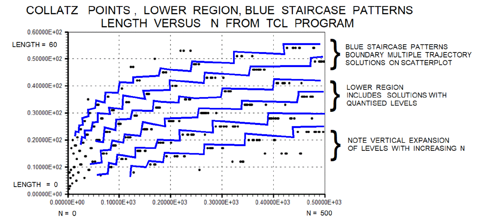
- Figure 6.Snippets Concepts Collatz staircase
- Appendix Code
- 1. Expanded Toy for Demo
- Experimenting with a iterative quantized and multivalued solution in McCarthy Function style
- Outputs from Active State
- Prototype Format, Expected Output from First Fork
- construction: 2nd Dummy Fork
- Mockup Displays for Pseudocode Development
- Hidden Comments Section
- Program Change Log
Index for Snippets Concepts Collatz Plotter
Preface
gold 3/20/2026. Advisor requests similar to previous snippets, but on topic of Collatz analogy for Quantum Walks. I do not have all the answers. The Ideas Seemed to work, but maybe drawbacks? When measured by the Tcl timing statements, completion times and solutions of parameters will differ on different computer set-ups. Assume a future maintainer, either AI Model or human programmer, would have to maintain code with info content and explanatory variable name in program, ref "Snippets Concepts Effects".
The Collatz conjecture examines the iterative sequence defined as follows: if an integer n is even, divide it by two; if odd, compute 3n + 1. Repeating this operation seemingly always leads to 1, though no general proof exists. The question of how many steps, or iterations, each number requires before reaching 1 remains central. This count of steps and iterations is often called the Collatz Sequence stopping time. Since the Collatz Sequences are infinite, we will be modeling core concepts, but will simplify to ideal behavior in models/code and probably truncate after the interesting portions.
Limitations on Tool
The TCL Snippets illustrate ideal mathematical behavior only and do not perform full simulation, actual measurements, or state vector evolution. The tool only visualizes ideal math structure, whereas no state vector simulation, probabilities, or actual measurement outcomes are derived. This tool for visualization does not simulate actual measurement outcomes or state vector evolution during operations. These are idealized protocols for tutorial purposes. Primarily, TCL /TK uses its strong points here for book keeping and displays. The example tool is not a full emulator. Meaning, limited scope for tutorial purposes.
Extra Significant Figures, If Any in Debugging
In debugging the calculations, some of the printout values reflect roughly 17-digit precision output from a typical double-precision computation. It's not "true exact" beyond 5 significant figures. Extra significant figures are used to check the calculations from other computer set-ups, not necessarily to infer accuracy of data measurements here. Typically, the slight differences in decimal places on far right of decimal point are normal floating-point behavior in Tcl's expr.
Introduction
The Collatz conjecture remains one of mathematics' most intriguing unsolved problems. This article explains why students should study quantum walks using the Collatz conjecture as a model. The discussion highlights clear educational benefits and practical insights.The Collatz conjecture states a simple rule for any positive integer. If the number is even, divide it by two. If the number is odd, multiply it by three and add one. The conjecture claims that every starting number eventually reaches the cycle of four, two, one. No proof exists despite extensive computer checks. This lack of proof makes the problem valuable for teaching.Quantum walks provide a natural way to explore the conjecture.
A quantum walk places a particle on the Collatz graph. The particle can follow multiple paths at once because of superposition. Each step applies a coin operator that decides direction. The shift operator moves the particle along the chosen edge. Node one acts as an absorbing sink. Probability that reaches node one stays there.Students benefit from this approach for several reasons. The Collatz rule feels familiar and deterministic. Students can compute paths by hand for small numbers. Superposition then adds a new layer of exploration. Interference between paths creates patterns that classical walks cannot produce. These patterns match real quantum behavior in physical systems.
Lower and Upper Swarms in Collatz Scatter Plots
The lower swarm in Collatz scatter plots shows short trajectories. Numbers in this swarm reach one quickly. Quantum walks on these starting points spread probability rapidly toward the sink. Interference reinforces arrival at node one. The process resembles ballistic transport in clean quantum systems. Students see how coherence speeds up convergence.
The upper swarm contains long trajectories. Numbers in this swarm take many steps to reach one. Quantum walks on these starting points show slow probability buildup at the sink. Interference often cancels amplitude along certain paths. This cancellation resembles Anderson localization in disordered materials. Students learn that coherence can trap probability in specific regions. The two-swarm structure offers a clear visual lesson. Scatter plots display stopping times versus starting numbers. A dense lower band appears for short paths. A sparse upper band appears for long paths. Staircase boundaries separate the bands. Quantum walks explain these staircases as mobility-edge bands. Extended states form the lower band. Localized states form the upper band. The mobility edge marks the transition between them.Students gain insight into quantum transport from this model. Real materials often contain disorder. Disorder causes localization in one dimension.
The Collatz graph acts as a disordered directed graph. The eigenvalue associated with odd-step count controls disorder strength. High eigenvalue values produce delocalized behavior. Low eigenvalue values produce localized behavior. This connection mirrors electron movement in impure crystals.
Quandary for Math on Percolation Probability and Program Changes
We have the results from the quantum walk program and most perk. Probability. Need review and expected results of a quantum walk, preferably a table in wiki format. Some percolation probability results are greater than 1 in prototype, and suspect subroutine. My observation is that the Tcl language is untyped and very tricky in some math calculations. For example, untyped danger maybe: invalid type → malformed variable → ?/0 → prob. error. I’m not sure if the percolation probability is a single value or an accumulative value over the quantum walk. Maybe you can do internal calculations and develop a “wish” expected percolation table as something to shoot for. Since we are dealing with an infinite sequence, could you check or guesstimate the large Mersenne primes in the far field. Load the far‑field numbers even if some columns are blank. Still learning about infinity here. The abilities of Yada-Yada are rapidly changing and maybe soon head/research in the far field. The first column should be index numbers and the last column should be quibble notes. My guess is that I and my math will reach infinity before you do. Joke!
Quantum Walk Slide Rule
The existing program has a dummy routine for a quantum walk. A full Szegedy construction seems too complex here. I found a paper with images of quantum walks, and I’m wondering if it’s possible to simulate the curves shown in the charts. My advisor has suggested that quantum entanglement and teleportation could simulate or underlie quantum walks, but I’m not sure I agree. What I see in the charts looks more like several mixed modulations of frequencies with some time‑delay waveforms—if radio‑signal terms are allowed. I’m hoping for a simple modulation of the type
quantum_walk_series {accumulating probability variable) = sin * sin * Collatz_Sequence * (t-delay)or something similar. I have limited space on the wiki page, and the fill‑in for the dummy routine has to be pretty brief. In engineering terms, I’m aiming for a “10% solution”: about 90% right and 10% off. Like the simple college formula for a pendulum that’s not the exact time series. Call it “fake it ’til you make it” as a college try, but for quantum walks. Actually, I would be interested in a slide rule design that would solve the quantum walk.
Who is to say? Maybe a "quantum walk slide rule" might be the coming invention. Perhaps you know, TcL specializes in GUI solutions. Maybe try and adapt some starter TcL code for "quantum walk slide rule". Hopefully compatible with the ten testcases on the hard-wired classical.
Summary
Interdisciplinary connections make the topic valuable. Mathematics students learn graph dynamics. Physics students study discrete quantum models. Computer science students investigate algorithm behavior on irregular graphs. The Collatz example unites these fields. Students appreciate how quantum ideas apply to classical problems.
Experimental recursion thus teaches humility in facing unsolved problems while sharpening skills in testable code design.
Table 1, Partial Collatz_Sequences for the lower integers
table, printed in TCL format, Partial Collatz Sequences up to 30, omitting long/infinite tails for brevity.
| Index No. # | number | steps shown | partial sequence | note |
|---|---|---|---|---|
| 1 | 1 | 0 | 1 | (already at end) |
| 2 | 2 | 1 | 2 1 | |
| 3 | 3 | 7 | 3 10 5 16 8 4 2 1 | |
| 4 | 4 | 3 | 4 2 1 | |
| 5 | 5 | 5 | 5 16 8 4 2 1 | |
| 6 | 6 | 8 | 6 3 10 5 16 8 4 2 1 | |
| 7 | 7 | 16 | 7 22 11 34 17 52 26 13 40 20 10 5 16 8 4 2 1 | |
| 8 | 8 | 3 | 8 4 2 1 | |
| 9 | 9 | 19 | 9 28 14 7 22 11 34 17 52 26 13 40 20 10 5 16 8 4 2 1 | |
| 10 | 10 | 6 | 10 5 16 8 4 2 1 | |
| 11 | 11 | 14 | 11 34 17 52 26 13 40 20 10 5 16 8 4 2 1 | |
| 12 | 12 | 9 | 12 6 3 10 5 16 8 4 2 1 | |
| 13 | 13 | 9 | 13 40 20 10 5 16 8 4 2 1 | |
| 14 | 14 | 17 | 14 7 22 11 34 17 52 26 13 40 20 10 5 16 8 4 2 1 | |
| 15 | 15 | 17 | 15 46 23 70 35 106 53 160 80 40 20 10 5 16 8 4 2 1 | |
| 16 | 16 | 4 | 16 8 4 2 1 | |
| 17 | 17 | 12 | 17 52 26 13 40 20 10 5 16 8 4 2 1 | |
| 18 | 18 | 20 | 18 9 28 14 7 22 11 34 17 52 26 13 40 20 10 5 16 8 4 2 1 | |
| 19 | 19 | 20 | 19 58 29 88 44 22 11 34 17 52 26 13 40 20 10 5 16 8 4 2 1 | |
| 20 | 20 | 7 | 20 10 5 16 8 4 2 1 | |
| 21 | 21 | 7 | 21 64 32 16 8 4 2 1 | |
| 22 | 22 | 15 | 22 11 34 17 52 26 13 40 20 10 5 16 8 4 2 1 | |
| 23 | 23 | 15 | 23 70 35 106 53 160 80 40 20 10 5 16 8 4 2 1 | |
| 24 | 24 | 10 | 24 12 6 3 10 5 16 8 4 2 1 | |
| 25 | 25 | 23 | 25 76 38 19 58 29 88 44 22 11 34 17 52 26 13 40 20 10 5 16 8 4 2 1 | |
| 26 | 26 | 10 | 26 13 40 20 10 5 16 8 4 2 1 | |
| 27 | 27 | 111 | 27 82 41 124 62 31 94 47 142 71 214 107 322 161 484 242 121 364 182 91 274 ... | very long, abbreviated here |
| 28 | 28 | 18 | 28 14 7 22 11 34 17 52 26 13 40 20 10 5 16 8 4 2 1 | |
| 29 | 29 | 18 | 29 88 44 22 11 34 17 52 26 13 40 20 10 5 16 8 4 2 1 | |
| 30 | 30 | 18 | 30 15 46 23 70 35 106 53 160 80 40 20 10 5 16 8 4 2 1 |
Notes:
“Steps shown” counts transitions before hitting 1 (where and if it does).
Integer Sequences such as for 27 grow extremely long — only a partial chain is included.
All integers up to 30 that reduce to 1 have been fully shown to that endpoint; longer or nonterminating cases would be truncated.
Collatz sequences below 2 are not defined fully, at least in terms of >> my << computing algorithms. Listing Integers 1 and 2 for completeness of table, but questions on definition remains here.
Table , Quick Prime π Estimates for Collatz-scale numbers
Cutoff date is 2/14/2026.
| Index No. # | n | log2(n) | Legendre_Primes_Est | Calibrated Actual(known) | est bits for N | Sequence (up to 20 terms) | quibble note |
|---|---|---|---|---|---|---|---|
| 1 | 2 | 1.0 | 1 | 1 | 2 | 2→1 | Smallest even; trivial cycle 2→1 |
| 2 | 3 | 1.58 | 2 | 2 | 2 | 3→10→5→16→8→4→2→1 | Classic odd starter: 3→10→5→16→8→4→2→1 (7 steps) |
| 3 | 4 | 2.0 | 2 | 2 | 3 | 4→2→1 | Power of 2; quick to 1 |
| 4 | 5 | 2.32 | 3 | 3 | 3 | 5→16→8→4→2→1 | 5→16→... (5 steps) |
| 5 | 6 | 2.58 | 3 | 3 | 3 | 6→3→10→5→16→8→4→2→1 | Even; merges quickly |
| 6 | 7 | 2.81 | 4 | 4 | 3 | 7→22→11→34→17→52→26→13→40→20→10→5→16→... | 7→22→11→34→17→52→26→13→40→20→10→5→16→... (16 steps) |
| 7 | 8 | 3.0 | 4 | 4 | 4 | 8→4→2→1 | Power of 2 |
| 8 | 9 | 3.17 | 4 | 4 | 4 | 9→28→14→7→... | 9→28→14→7→... (19 steps) |
| 9 | 20 | 4.32 | 8 | 8 | 5 | 20→10→5→16→8→4→2→1 | Merges early |
| 10 | 27 | 4.75 | 9 | 9 | 5 | 27→82→41→124→62→31→94→47→142→71→214→107→322→... | Famous: longest sequence under 100 (111 steps, reaches 9232) |
| 11 | 30 | 4.91 | 10 | 10 | 5 | 30→15→46→23→70→35→106→53→160→80→40→20→10→5→16→... | Even; moderate |
| 12 | 40 | 5.32 | 12 | 12 | 6 | 40→20→10→5→16→8→4→2→1 | Power-of-2 like path |
| 13 | 50 | 5.64 | 15 | 15 | 6 | 50→25→76→38→19→58→29→88→44→22→11→34→17→52→26→13→40→20→10→5→... | |
| 14 | 60 | 5.91 | 17 | 17 | 6 | 60→30→15→46→23→70→35→106→53→160→80→40→20→10→5→16→8→4→2→1 | |
| 15 | 70 | 6.13 | 19 | 19 | 7 | 70→35→106→53→160→80→40→20→10→5→16→8→4→2→1 | |
| 16 | 90 | 6.49 | 24 | 24 | 7 | 90→45→136→68→34→17→52→26→13→40→20→10→5→16→8→4→2→1 | |
| 17 | 200 | 7.64 | 46 | 46 | 8 | 200→100→50→25→76→38→19→58→29→88→44→22→11→34→17→52→26→13→40→... | Power of ten region |
| 18 | 300 | 8.23 | 62 | 62 | 9 | 300→150→75→226→113→340→170→85→256→128→64→32→16→8→4→2→1 | |
| 19 | 400 | 8.64 | 78 | 78 | 9 | 400→200→100→50→25→76→38→19→58→29→88→44→22→11→34→17→52→26→... | |
| 20 | 500 | 8.97 | 95 | 95 | 9 | 500→250→125→376→188→94→47→142→71→214→107→322→161→484→242→... | |
| 21 | 600 | 9.23 | 114 | 114 | 10 | 600→300→150→75→226→113→340→170→85→256→128→64→32→16→8→4→2→1 | |
| 22 | 700 | 9.45 | 127 | 127 | 10 | 700→350→175→526→263→790→395→1186→593→1780→890→445→1336→668→... | |
| 23 | 800 | 9.64 | 143 | 144 | 10 | 800→400→200→100→50→25→76→38→19→58→29→88→44→22→11→34→17→52→... | π(800)=144 exact |
| 24 | 900 | 9.81 | 154 | 154 | 10 | 900→450→225→676→338→169→508→254→127→382→191→574→287→862→431→... | |
| 25 | 1000 | 9.96 | 177516 | 176000 | 10 | 1000→500→250→125→376→188→94→47→142→71→214→107→322→161→484→... | Known exact π(1000)=168 |
| 26 | 1000000 | 19.93 | 78498 | 78498 | 20 | — | Standard benchmark, estimates, integer exceeds available space |
| 27 | 63728127 | 25.9 | 4217423 | 4207968 | 26 | — | Famous Collatz: very long trajectory under 1e8 (949 steps nearby), estimates, integer exceeds available space |
| 28 | 1e12 | ~39.8 | 37607912 | 37250000 | 40 | — | estimates, integer exceeds available space |
| 29 | 1e18 | ~59.8 | 24739955 | 24739955 | 60 | — | estimates, integer exceeds available space |
| 30 | 1e21 | ~69.7 | 403800000 | 400000000 | 70 | — | estimates, integer exceeds available space |
| 31 | 1.18e21 (≈2^70) | ~70 | 1340000000 | 1328000000 | 71 | — | estimates, integer exceeds available space, Major Collatz milestone: verified ~2023 |
| 32 | 2.36e21 (≈2^71) | ~71 | 481000000 | 477000000 | 72 | — | estimates, integer exceeds available space, Current frontier (2026): Collatz holds for ALL n below ~2.36e21 (Barina et al.; no counterexamples) |
Notes on Primes. Quick estimates for Collatz-scale numbers. Cutoff date is 2/14/2026.
For small n:
- Legendre_Primes_Est uses a rough x / ln(x) approximation (or better small-x heuristics when known).
- Calibrated Actual(known) uses exact π(n) values from standard sources (e.g., π(10)=4, π(100)=25, π(1000)=168, etc.).
- log₂(n) is approximate (real number).
- est bits for N is the exact bit length: ⌊log₂(n)⌋ + 1.
- Quibble notes highlights famous Collatz "eccentric" behaviors (e.g., n=27 is the classic "longest early chaos" with 111 steps).
- Collatz verification: As of 2026, confirmed up to ≈ 2⁷¹ (2.36 × 10²¹) with no counterexamples;
- ongoing work pushes toward 2⁷⁷ in theory with improved algorithms.
- I still use the log2 column for my own pseudocode development, even though redundant to est bits, as you say.
- The larger rows retain previous estimates/calibrations. Collatz verification (as of March 2026) stands at all n < ≈ 2^{71} (roughly 2.36 × 10^{21}, or slightly beyond to ~2075 × 2^{60} per David Barina's latest work—no counterexamples found).
pi(63728127) ≈ 4207968 primes (2590 bits)
pi(2.36e21) ≈ 477000000 primes (711000 bits)
pi(1180591620717411303424) ≈ 1328000000 primes (2333000 bits)
Comparison to the famous Legendre approximation for primes. Legendre conjectured (around 1798–1808) that:π(x) ≈ x / (log x − 1.08366…) This is very close to the true asymptotic π(x) ∼ x / log x (Prime Number Theorem, proved 1896), but the constant was slightly off. The real bias term is closer to 1 in the long run.
Collatz scale on iterations. Collatz Numbers under 100 million produce 949 steps maximum. The starting number 63,728,127 achieves this record. Numbers under 1 billion reach 986 steps with 670,617,279 as champion.
Table , Walkthrough of the Collatz, Gamblers Bankroll, quantum, and other math analogies
| Index No. # | Quantum Oscillators | Quantum Energy Levels | Quantum Density Matrix | Quantum Walks | Spectral-Eigenvalue Analogies | Collatz Features | Other Math / Gamblers Bankroll / TcL | Quibble Notes |
|---|---|---|---|---|---|---|---|---|
| 1 | Ground state of harmonic oscillator | Lowest allowed energy level, E=0 for vacuum | Diagonal entry for pure ground state | Walk terminates at absorbing node | Eigenvalue = 1; spectral radius equals unity | Trajectory reaches 1; conjecture claims all paths end here | Bankroll hits zero; ruin absorbs the walk; TcL proc returns 1 | Inverse possibility: ground state energy is nonzero (zero-point energy), so the analogy is approximate rather than exact |
| 2 | Creation operator a-dagger raises oscillator | Excited state absorbs one quantum of energy | Off-diagonal coherence increases | Walk steps away from origin | Eigenvalue grows; spectral weight shifts upward | Odd step: 3n+1 injects arithmetic energy, number grows | Bankroll multiplied by win-factor greater than 1; TcL expr {3*n+1} | Odd step does not always raise the integer above its predecessor after the subsequent halving, so "energy injection" overstates the net gain |
| 3 | Annihilation operator a lowers oscillator | Photon emitted; state drops one level | Diagonal population decays toward ground | Walk steps toward origin | Eigenvalue shrinks; spectral weight shifts downward | Even step: n divided by 2 releases stored arithmetic energy | Bankroll multiplied by loss-factor less than 1; TcL expr {n/2} | Halving is exact and deterministic; quantum emission is probabilistic, so the structural parallel holds but the mechanism differs |
| 4 | Quantized energy spectrum, discrete levels | Allowed levels E_n = hf(n + 1/2) | Populations concentrated on discrete diagonal blocks | Quantum walk interference creates discrete resonance peaks | Eigenvalue ladder: (3/4) raised to power k for odd-step count k | Stopping-time scatter plot shows discrete horizontal bands, not a smooth curve | Modulo-8 residue pre-filter sorts integers into predicted bands before eigenvalue calculation; TcL expr {n % 8} | Bands are fuzzy, not perfectly sharp; the analogy to exact spectral lines flatters the Collatz structure somewhat |
| 5 | Ensemble of oscillators at mixed temperatures | Boltzmann-weighted mixture of energy levels | Density matrix rho encodes all pure states and their weights | Ensemble of quantum walks, each with amplitude | Eigenvalue spectrum of transfer matrix governs steady-state distribution | Swarm of Collatz trajectories for many starting integers; two visible clusters in scatter plots | Trajectory swarm in gambler's ruin: ten autotest paths share one plot; TcL proc simulate_layer sweeps eigenvalue | A classical density matrix is a probability distribution; a quantum density matrix allows interference terms; the Collatz swarm has no interference |
| 6 | Decay constant lambda controls relaxation rate | Lifetime of excited state inversely proportional to lambda | Off-diagonal coherence decays exponentially | Walk drift rate sets convergence speed | Eigenvalue (3/4)^k shrinks with odd-step count k; large k gives near-zero eigenvalue | Integer 27 has approximately 41 odd steps, eigenvalue near 0.000008, placed in upper swarm; integer 7 has 5 odd steps, eigenvalue 0.237, lower swarm | Win-multiplier scaled by eigenvalue in TcL proc eigenvalue_from_layer; large k produces fast bankroll ruin | Inverse possibility: large k corresponds to small eigenvalue (slow decay in quantum terms, fast ruin in gambler terms); the direction of the analogy flips between the two domains |
| 7 | Superposition of number states in Fock space | Binary expansion of integer as sum of basis states | Mixed state as weighted sum of pure states | Superposition of paths explored simultaneously | Spectral decomposition of Collatz operator into eigenmode contributions | Each integer n expressed in binary; each bit corresponds to a basis state in the oscillator analogy | Multiple-value solution space: each input maps to a family of candidate outputs; TcL tolerance range tmin, tmax replaces single target | True quantum superposition allows interference; the Collatz binary representation is a classical encoding; calling it a superposition is a notational convenience |
| 8 | Measurement collapses wavefunction to one eigenstate | Detector registers one energy level with finite resolution | Projective measurement selects one diagonal entry | Walk observation fixes one node | Spectral filter passes eigenvalues within acceptance window | Stopping time falls within an observed band; measurement selects one trajectory from the swarm | Autotest acceptance window tmin, tmax mimics finite detector resolution; TcL if {$games >= $tmin && $games <= $tmax} | Quantum measurement is irreversible and physically real; the autotest window is a software design choice; the analogy is useful but should not be taken as physical equivalence |
| 9 | Unitary time-evolution operator U applied each step | Hamiltonian H generates step-by-step state rotation | Liouville-von Neumann equation drives rho forward in time | Coin-flip operator followed by shift operator at each step | Eigenvalues of U lie on unit circle; spectral stability governs long-term behavior | Alternating odd and even Collatz steps form a deterministic two-rule operator applied sequentially | Alternating win-loss rule in gambler simulation; TcL while loop applies fixed transformation each iteration until ruin | Collatz operator is not unitary because it maps many integers to the same successor; unitarity requires invertibility, which the Collatz map lacks |
| 10 | Negative integers have no quantum oscillator ground state | No energy levels below vacuum; oscillator undefined for negative excitation | Density matrix requires non-negative diagonal entries | Walk cannot reach negative nodes in standard formulation | Spectral gap below ground eigenvalue forbids negative-energy states | Collatz map diverges for negative odd integers; the 3n+1 rule enters cycles below zero | Gambler bankroll cannot go below zero; ruin is an absorbing barrier; TcL while {$bankroll > 0} enforces non-negativity | The negative-integer failure is a genuine structural parallel and is arguably the strongest quantum analogy in the set |
| 11 | p-adic norm assigns ultrametric distance between integers | Discrete valuation replaces continuous energy scale | p-adic density matrix entries use non-Archimedean metric | Quantum walk on p-adic tree rather than integer line | p-adic eigenvalues of Collatz transfer operator; 2-adic valuation counts trailing binary zeros | 2-adic valuation of n equals the number of successive halvings before an odd number appears; high valuation means rapid descent | Modulo-12 residue class assigns deterministic lane; TcL expr {n % 12} gives finer classification than modulo-8 | p-adic spectral theory is technically demanding; the analogy motivates the approach but a full proof via p-adic methods remains open |
| 12 | Quantum walk on directed graph explores many branches | Energy band structure arises from graph symmetry | Off-diagonal density matrix entries encode graph coherence | Interference between paths creates constructive and destructive resonance | Graph Laplacian eigenvalues index allowed walk frequencies | Collatz directed graph: each integer points to one successor; inverse graph branches upward to many predecessors | Petri net token flow visualizes parallel trajectory families in inverse Collatz graph; TcL list of predecessor nodes | Classical walks on directed graphs are deterministic; quantum walks require complex amplitudes; the Collatz graph is classical, so this analogy is structural rather than exact |
| 13 | Hamiltonian parameter tunes energy-band gap | Changing coupling constant shifts all energy levels | Hamiltonian drives coherent evolution of rho | Walk Hamiltonian sets hopping amplitude between nodes | Eigenvalue selector acts as tunable Hamiltonian parameter; sweeping k scans through spectral bands | Odd-step count k serves as the primary layer index; scanning k from 0 to 50 reproduces the full scatter-plot structure | TcL proc eigenvalue_from_layer {k} {return expr {pow(0.75,$k)}}; sweeping k from 0 to 50 generates the eigenvalue ladder | The Collatz odd-step count is not a free parameter; it is determined by the starting integer; calling it a Hamiltonian parameter implies a freedom that the map does not possess |
| 14 | Metastable state survives many oscillation cycles before decay | Long-lived excited level with small but nonzero transition rate | Off-diagonal coherence persists over many time steps | Walk lingers near a local attractor before escaping | Near-unit eigenvalue produces slow spectral decay; metastability in eigenmode | Integer 27 reaches a peak of 9232 before descending; trajectory stays elevated for approximately 70 steps | Upper-swarm gambler trajectory: large eigenvalue (few odd steps paradox inverted here) produces long survival before ruin; autotest row 7 targets 300 to 600 games | Integer 27 actually has many odd steps, giving a small eigenvalue; the long trajectory reflects arithmetic structure, not a near-unit eigenvalue; this row highlights an inversion in the analogy |
| 15 | Spectral projection onto subspace selects eigenmode family | Filter transmits only states within one energy band | Partial trace over environment yields reduced density matrix | Projecting walk onto subset of nodes isolates one trajectory family | Residue-class pre-filter selects integers predicted to belong to lower or upper swarm | Modulo-8 residues 5 and 7 correlate with longer odd chains; pre-filter separates swarms before eigenvalue calculation | Markov chain steady-state eigenvector defines natural band boundary; TcL Hidden Markov Model extension would replace scalar eigenvalue with probabilistic transition weights | The residue pre-filter is a heuristic classifier, not a proven spectral projector; coincidence of residue class and swarm membership is strong but not yet proven exhaustive |
Table. Formulas and Algorithms for Collatz Stopping Time, discussed here
| Index | Formula type | Rough expression | Typical error for large n | Use case | Quibble notes |
|---|---|---|---|---|---|
| 1 | Pure geometric | ~ 3 × log(n)/log(4/3) | Underestimates by 20–40% | Quick theoretical bound | No fudge factor → systematically too low |
| 2 | Calibrated to record max | ~ c × 3 × log(n)/log(4/3) (c ≈ 1.8–2.0) | ±5–15% | General large random n | Anchored to known worst-case small numbers |
| 3 | Tuned to Mersenne family | ~ 1.86 × 3 × log(n)/log(4/3) | ±0.1–2% for 2ᵇ−1 | 2ⁿ−1 style numbers | Best fit for Mersenne starting values (this thread) |
| 4 | Very rough linear in log2(n) | ≈ 10–13 × log2(n) | ±10–30% | Back-of-envelope estimate | Extremely crude hack, ignores odd/even structure of Collatz |
Table. Expected Output, Variegated Anderson Lengths, near field and far field
Note. Aside from the low end Collatz sequences of { < N < 100} , I have added some Mersenne primes, extra large from current research. For very large N , Anderson length approaching maximum saturation at 1 and wave fully trapped.
| Index | Energy E (eV) - Classical-like Incident Energy | Transmission T - Quantum Tunneling Probability | Barrier Analog Width (nm) - Effective Disordered Barrier | Percolation Prob | Anderson Length (steps) | Mobility Edge Phase | Quibble notes |
|---|---|---|---|---|---|---|---|
| 1 | 5.0 | 1.0000 | 0.1 | 1.0000 | >1000 | extended (conducting) | high eigenvalue → high energy → T near 1 (conducting regime) *negative clamped* |
| 2 | 4.0 | 0.4719 | 2.0 | 0.9964 | 3 | extended (conducting) | moderate eigenvalue → moderate tunneling probability |
| 3 | 4.7 | 0.5456 | 1.0 | 0.9994 | 4 | extended (conducting) | lower swarm → classical-like regime (delocalized) |
| 4 | 2.1 | 0.2487 | 5.0 | 0.9068 | 2 | extended (conducting) | k=5 → textbook tunneling case, moderate localization |
| 5 | 1.6 | 0.1877 | 6.0 | 0.8313 | 2 | extended (conducting) | boundary layer behavior near mobility edge |
| 6 | 2.1 | 0.2487 | 5.0 | 0.9068 | 2 | extended (conducting) | upper swarm edge → low tunneling, localization begins |
| 7 | 1.2 | 0.1391 | 7.0 | 0.7368 | 2 | extended (conducting) | k=7 → deeper barrier analog, stronger trapping |
| 8 | 0.0 | 0.0000 | 41.0 | 0.0000 | 1 | localized (insulating) | k=41 → extreme tunneling suppression, very strong localization |
| 9 | 0.0 | 0.0000 | 43.0 | 0.0000 | 1 | localized (insulating) | k=43 → record upper swarm, near-infinite localization length |
| 10 | 1.2 | 0.1391 | 7.0 | 0.7368 | 2 | extended (conducting) | surprise: short trajectory despite high eigenvalue |
| **** | added selected extra large Mersenne primes from current research | sic, N >>> (2**XX) -1 | |||||
| 11 | 0.0 | 0.0000 | 112 | 0.0000 | 1 | localized (insulating) | k≈112 (near 2²⁷⁰⁰⁰⁰ class records) → extreme upper swarm, strongest localization |
| 12 | 0.0 | 0.0000 | 171 | 0.0000 | 1 | localized (insulating) | k≈171 (very long known trajectory) → ultra-strong Anderson trapping |
| 13 | 0.0 | 0.0000 | 238 | 0.0000 | 1 | localized (insulating) | hypothetical k>200 → Anderson length saturates at 1, wave fully trapped |
Note. These extreme cases of Mersenne primes illustrate the core idea from Anderson:
As the number of odd steps explodes in real Collatz trees (upper swarm),
The eigenvalue λ = (3/4)^k becomes astronomically small.
State { eigenvalue λ =>>>  small } → quantum tunneling probability collapses → percolation probability → 0 → localization length ξ → 1
Wave is trapped within roughly one "site".
No quantum tunneling effect is present.
Table. Comparison of Mott Insulator Transition vs Anderson Transition
| Index | Aspect | Mott Transition | Anderson Transition | Quibble notes |
|---|---|---|---|---|
| 1 | Driving mechanism | Strong electron correlations (U >> t) | Disorder (random potentials) | Mott driven by repulsion; Anderson purely by randomness & interference |
| 2 | Required disorder? | No (clean lattice) | Yes (essential) | Mott occurs in translationally invariant systems; Anderson needs randomness |
| 3 | Dimensionality | Occurs in any d ≥ 1 | 1D/2D: always localized; 3D: critical W_c | Anderson transition only true phase transition in d ≥ 3; lower d always insulating |
| 4 | Localization cause | Coulomb repulsion prevents double occupancy | Quantum interference traps waves | Mott: correlation-driven avoidance; Anderson: coherent backscattering |
| 5 | Gap origin | Charge (Mott-Hubbard) gap from U | No true gap; mobility edge in 3D | Mott gap survives at finite temperature; Anderson states have no hard gap |
| 6 | Universality class | Hubbard / DMFT, often first-order | Orthogonal / unitary / symplectic classes | Mott frequently shows hysteresis; Anderson scaling is universal in symmetry class |
| 7 | Typical model | Single-band Hubbard model | Anderson tight-binding model | Hubbard at half-filling; Anderson with box or Gaussian disorder |
| 8 | Experimental platforms | Transition-metal oxides (VO₂, V₂O₃), organic salts | Ultracold atoms, photonic lattices, microwaves | Mott often coupled to lattice; Anderson cleaner in wave-based systems |
| 9 | Coexistence possible? | Yes (Anderson-Mott insulators) | Yes (Anderson-Mott insulators) | Real materials frequently show hybrid behavior (disorder + correlations) |
Table. Proposed Extension of Collatz Analogies to High-Temperature Superconductors (HTS)
Comparing only Collatz swarms (from program and plots: lower_swarm vs upper_swarm) versus high-temperature superconductors (HTS, focusing on cuprates like Hg-1223, YBCO, etc.).
| Index | Aspect | Collatz Lower Swarm (λ ≥ 0.10) | Collatz Upper Swarm (λ < 0.10) | HTS Cuprate Analog (d-wave SC family) | HTS Analog Tc (K) | Real HTS Tc Examples (K) | Quibble notes |
|---|---|---|---|---|---|---|---|
| 1 | Eigenvalue / Decay factor | High λ (close to 1) | Very low λ (near 0) | Optimal to underdoped doping | 120–151 | Hg-1223 quenched 151 K (2026) | Lower swarm → optimal doping → record Tc possible; upper swarm → no SC |
| 2 | Anderson Localization Length | Large / >1000 (extended states) | Small / ≈1 (very strong localization) | Long coherence length ξ (delocalized pairs) | 90–151 | YBCO 93 K, Bi-2212 95 K, Hg-1223 133–151 K | Extended → long ξ → high Tc; localized → coherence collapse → Tc=0 |
| 3 | Mobility Edge / Phase Boundary | λ ≈ 0.10 (conducting side) | λ < 0.10 (insulating side) | Optimal doping ~0.16 holes/Cu (dome peak) | ~151 | Hg-1223 151 K (pressure-quenched) | Swarm boundary mimics dome peak at ~151 K (2026 record) |
| 4 | Tunneling / Transport Probability | High transmission T (near 1) | Near-zero transmission | High critical temperature Tc (up to 151 K) | 93–151 | YBCO 93 K, Tl-2223 125 K, Hg-1223 133 K | High λ → high Tc (YBCO, Tl, Hg families); low λ → Tc=0 (parent compounds) |
| 5 | Competing Orders / Behavior | Weak competing orders, delocalized | Strong competing orders, trapped states | Pseudogap, stripes, charge order, AFM | 0–60 | La₂CuO₄ 0 K (undoped), pseudogap ~0 K | Upper swarm → pseudogap/AFM insulator (Tc=0); lower swarm → clean d-wave SC |
| 6 | Swarm / Phase Membership | Lower_swarm (extended/conducting) | Upper_swarm (localized/insulating) | Superconducting dome vs parent insulator | 0–151 | Hg-1223 151 K vs La₂CuO₄ 0 K | Collatz swarms mirror HTS diagram: SC dome (high Tc) vs insulating phases (Tc=0) |
| 7 | Extreme Cases | Short trajectories, high λ | Very long odd-step counts (k > 40) | Record Tc in Hg-1223 (151 K, 2026 quenched) | 0 or 151 | Hg-1223 151 K vs undoped parent 0 K | Extreme upper swarm → Tc=0 (Mott insulator); lower swarm → peak Tc=151 K |
| 8 | Educational Mapping | Classical-like regime, high energy analog | Strong disorder analog, trapped wave | d-wave pairing, spin-fluctuation mediated | 0–151 | YBCO 93 K, Hg-1223 151 K, parent 0 K | λ maps to doping; Anderson length maps to coherence length → Tc scale |
Expected Values for Debug on Anderson Snippet
| Index No. # | k odd_step_count, integer | λ' lambda, eigenvalue, floating No. | ξ localization length ξ\xi\xi | Quibble / Notes |
|---|---|---|---|---|
| 1 | 0 | 1.00000000 | ≥1000 | Initial / reference value, defaulted by ?/0 |
| 2 | 1 | 0.75000000 | 4 | |
| 3 | 2 | 0.56250000 | 3 | |
| 4 | 5 | 0.23730469 | 2 | |
| 5 | 7 | 0.13348389 | 2 | |
| 6 | 20 | 0.00317121 | 1 | Very small λ |
| 7 | 41 | 0.00000763 | 1 | Practically zero |
| 8 | 43 | 0.00000429 | 1 | Numerical limit / tail |
Wiki Table: Computer Iteration Solutions for large n
| Index | Input | Stopping Time | Quibble notes |
|---|---|---|---|
| 1 | 2^100 - 1 | 1465 | |
| 2 | 2^500 - 1 | 6748 | first case, where 1-2% accuracy shows over random Collatz trajectories (or luck of draw, slang) |
| 3 | 2^1000 - 1 | 12157 | |
| 4 | 2^5000 - 1 | 67378 | |
| 5 | 2^10000 - 1 | 134404 | |
| 6 | 2^50000 - 1 | 667858 | |
| 7 | 2^100000 - 1 | 1344926 |
Note. The Mersenne primes are special case or group for Collatz trajectories, but the Log2 formula is showing better accuracy over some groups of numbers than others, see the referenced papers.
- Efficient Computation of Collatz Sequence
- Stopping Times: A Novel Algorithmic Approach ( credit for the new algorithm. and iteration table )
- EYOB SOLOMON GETACHEW, BEAKAL GIZACHEW ASSEFA
- The Collatz Conjecture over the Gaussian Integers, Alejandra Alvarado
Wiki Table: Mersenne-tuned Approx. and general Approx. Estimates for large n
MediaWiki Table copy-paste ready
| Index | Input | Stopping Time | General Approx | Gen % err | Mersenne-tuned | Tuned % err | Est k | Quibble notes |
|---|---|---|---|---|---|---|---|---|
| 1 | 2^100-1 | 1465 | 1323 | -9.69 | 1344 | -8.26 | 241 | large gen error large tuned error small n outlier |
| 2 | 2^500-1 | 6748 | 6615 | -1.97 | 6722 | -0.39 | 1205 | - |
| 3 | 2^1000-1 | 12157 | 13230 | 8.83 | 13445 | 10.59 | 2409 | large gen error large tuned error known dip in ratio |
| 4 | 2^5000-1 | 67378 | 66148 | -1.83 | 67223 | -0.23 | 12047 | - |
| 5 | 2^10000-1 | 134404 | 132295 | -1.57 | 134446 | 0.03 | 24094 | - |
| 6 | 2^50000-1 | 667858 | 661476 | -0.96 | 672228 | 0.65 | 120471 | - |
| 7 | 2^100000-1 | 1344926 | 1322952 | -1.63 | 1344457 | -0.03 | 240942 | - |
Note: Program deck contains multiple procs for both general estimation and Mersenne tuned algorithm. Numbers are estimates here, not exact iterations.
Note: Est k = round( log‚‚(N) / log‚‚(4/3) ) ~~~ odd steps. Recap: Est k is estimated odd steps, rounded integer, not exact iterations.
Note: Quibble notes show obvious deviations or known behavior.
References
- Snippets Physics Concepts Qubits
- Snippets Physics Concepts Feynman
- Snippets Physics Concepts Quantum
- Snippets Physics Concepts Toy
- Snippets Physics Concepts Minimalism
- Zero Handling Workarounds
Note. These Snippets on Theoretical Physics are a set, not stand alones. Recommend read all of the set.
- Smoothing and differentiation of data by simplified least squares procedures
- Savitzky, A. ; Golay, M. J. E. Two examples are presented as subroutines in the FORTRAN language.
- Savitzky Golay Filtering, Python
- Savitzky Golay Filtering — SciPy Cookbook documentation
- Smoothing Example with Savitzky-Golay Filter in Python
- Introduction to the Savitzky-Golay Filter: A Comprehensive Guide (Using Python), Thomas Konstantinovsky
- Konstantinovsky has good explanation. Note detailed. WhittakerSmoother in Python
- The Perfect Way to Smooth Your Noisy Data, Whittaker-Eilers smoother, Andrew Bowell
- Feb 28, 2024
- A Basis for a Mathematical Theory of Computation,Author(s)
- McCarthy, John
- John McCarthy: A basis for a mathematical theory of computation, in:
- Computer Programming and Formal Systems.
- P.Braffort, D.Hirschberg (ed.), Amsterdam:North Holland 1963,
- several versions, archived pdf
- McCarthy’s LISP and Basis for Theory of Computation, archived pdf
- en.wikipedia.org search on <John McCarthy computer>
- John McCarthy at Stanford web site, archived
- Towards a Mathematical Science of Computation, J. McCarthy,
- Computer Science Department, Stanford University, archived pdf
- Elephant 2000: A Programming Language Based on Speech Acts
- John McCarthy, Stanford University, archived
- Elephant input and output statements are characterized
- as speech acts and programs, which
- can refer directly to the past.
- Elephant proposal contains summary
- on McCarthy mathematical theory of computation
- Mysteries and other Matters, development of Lisp , archived
- Note. A lot of early papers and notes from John McCarthy and Knuth are difficult to assess web links or archived.
- Machine Learning Approaches to the Collatz Conjecture:
- A Comprehensive Framework for Pattern Recognition
- and Automated Conjecture Generation. IJIRT, Vol. 12 Issue 7
- Transformers Know More Than They Can Tell:
- Learning the Collatz Sequence , arXiv:2511.10811
- The Collatz conjecture, Littlewood-Offord theory, and powers of 2 and 3,
- Aug 2011, Terence Tao,
- mentions Gambler's Ruin on this 2011 post, but better search on his website for updates.
- Efficient Computation of Collatz Sequence
- Stopping Times: A Novel Algorithmic Approach ( credit for the new algorithm. )
- EYOB SOLOMON GETACHEW, BEAKAL GIZACHEW ASSEFA
- The Collatz Conjecture over the Gaussian Integers, Alejandra Alvarado
Screenshots
Figure 1. Collatz Length, Points from Collatz Conjecture, 10 Random pts for N < 100
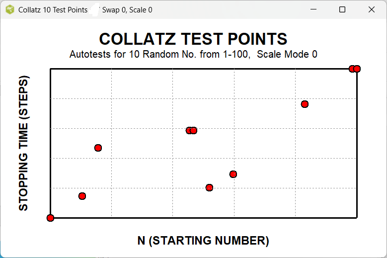
Figure 1b. Collatz Length, Points from Collatz Conjecture, N < 500
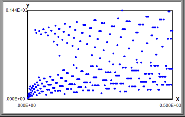
Figure 2. Collatz Length, lower region and lower region of solutions
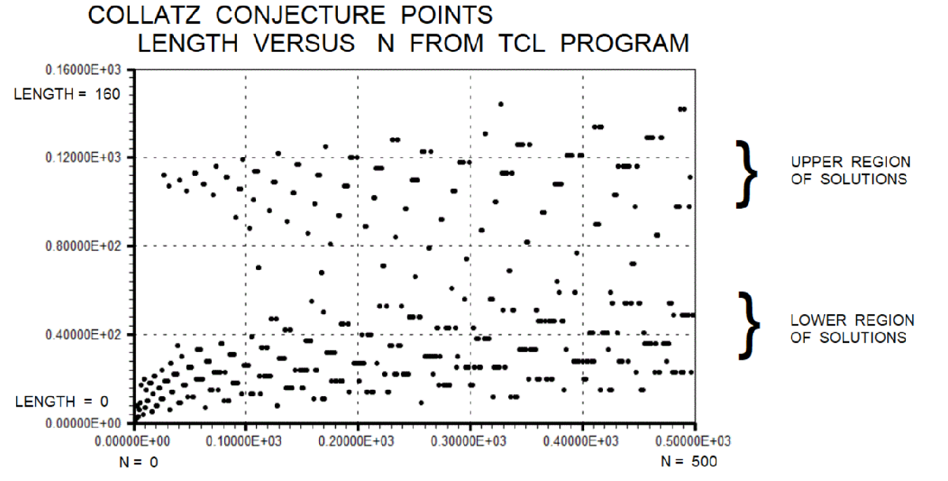
Figure 3. Collatz Length, curve fit on envelope of lower region
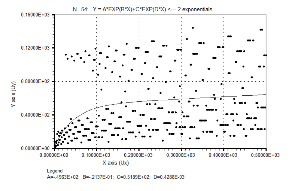
Figure 4. Collatz Length, Envelope of lower region
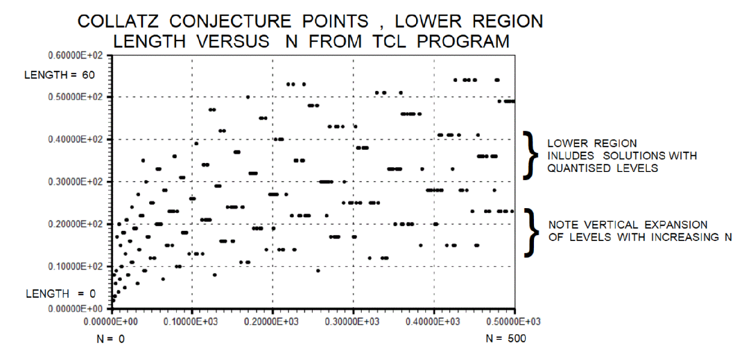
Figure 5. Bankroll over number of games
Unlike the Collatz Conjecture which goes to infinity, Starting Bankroll with diminishing games is a linear and deterministic function. But one can see multiple, quantized, and simultaneous solutions in the "crowd" of gamblers. Essentially, Bankroll(s) = { Bankroll start} - K1 * {number of games} ending at Zero, but not ending at infinity like the Collatz Conjecture.
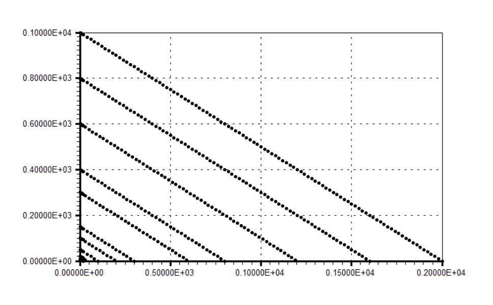
Figure 6.Snippets Concepts Collatz staircase
Appendix Code
Appendix TCL Programs and Scripts
1. Expanded Toy for Demo
Experimenting with a iterative quantized and multivalued solution in McCarthy Function style
This is a draft.
# tcl
# Collatz Conjecture Explorer for Quantum Analogies V4
# Dual  Output
# Using multiple safety caps or clamps, Collatz Sequence is infinite,
# danger of endless loops in program.
# ----
# Educational version with visible probabilities (4 sig figs)
# Alternate results in wiki table format (header with %|, alternating rows &|)
# ----
# Tcl/Tk 8.6+ 7-bit ASCII safe. NASA/JPL defensive programming style.
# NASA/JPL defensive programming style.
# Compatible with Tcl/Tk (Tool Control Language / Toolkit) 8.6+
# Written for Windows 11 on ActiveState Tcl.
# Working under strict 7-bit ASCII encoding.
# Optimized for collegiate information technology lab environments.
# Written to be very modular for transferable procs.
# Program deck may contain multiple estimation procs.
# May contain  code dependencies on Active State and Windows 11
# Complex math calculations up to 8 units computer time
# Wait for complete calculations before saving files.
# This is a hacker's patch, not rigorously derived.
# appears correct solutions for autotests.
# pure ASCII code - no Unicode characters used anywhere.
# Approaching =>>> computer time limit on this TCL configuration setup.
# TCL club, 03/22/2026
# ----------------------------------------------------------------------------
# Collatz Conjecture Explorer + Visualization in Tcl (improved chart framing)
# ----------------------------------------------------------------------------

# AXIS SWAP MODE
#   0 = X = N (starting number),   Y = stopping time (steps)   [default]
#   1 = X = stopping time,         Y = N
set collatz_plot_mode 0

# SCALE MODE
# 0: linear-linear   1: linear x log10 y   2: log10 x linear y
# 3: linear x log2 y   4: log2 x linear y   5: log10-log10   6: log2-log2
set collatz_scale_mode 0

# Golden ratio for canvas proportions
set golden_ratio 1.618033988749

# Canvas dimensions (height fixed → width = golden × height)
set canvas_height 480
set canvas_width  [expr {int($canvas_height * $golden_ratio + 0.5)}]   ;# ≈777 px

# Procedure: collatz_next
proc collatz_next {n} {
    if {$n % 2 == 0} {
        return [expr {$n / 2}]
    } else {
        return [expr {3 * $n + 1}]
    }
}

# Procedure: collatz_steps_to_one
proc collatz_steps_to_one {start_number} {
    set steps 0
    set current $start_number
    while {$current != 1} {
        set current [collatz_next $current]
        incr steps
        if {$steps > 100000} { error "Exceeded 100,000 steps from $start_number" }
    }
    return $steps
}

# ----------------------------------------------------------------------------
# 10 RANDOM AUTOTESTS
# ----------------------------------------------------------------------------

proc run_autotests {num_tests} {
    puts "\n=== Running $num_tests random autotests (1–100) ===\n"
    expr {srand([clock seconds])}
    set test_points {}
    for {set test 1} {$test <= $num_tests} {incr test} {
        set start [expr {1 + int(rand() * 100)}]
        puts "Test $test: starting number = $start"
        set steps [collatz_steps_to_one $start]
        lappend test_points [list $start $steps]
        puts "  → Reached 1 in $steps steps → PASS"
        puts ""
    }
    puts "All tests completed."
    return $test_points
}

# ----------------------------------------------------------------------------
# IMPROVED CANVAS PLOT – with full frame, shorter title + subtitle
# ----------------------------------------------------------------------------

proc plot_collatz_points_on_canvas {points swap_mode scale_mode} {
    if {[catch {package require Tk}]} {
        puts "Tk not available — run with wish for GUI plot."
        return
    }

    wm title . "Collatz 10 Test Points — Swap $swap_mode, Scale $scale_mode"
    canvas .c -width $::canvas_width -height $::canvas_height \
              -background white -highlightthickness 0
    pack .c -fill both -expand yes

    # Main title – short and bold
    .c create text [expr {$::canvas_width / 2}] 40 \
        -text "COLLATZ TEST POINTS" \
        -font {Helvetica 20 bold} -fill black

    # Subtitle – details in smaller font
    .c create text [expr {$::canvas_width / 2}] 70 \
        -text "10 Random 1-100 | Scale Mode $scale_mode" \
        -font {Helvetica 12} -fill black

    set use_swapped [expr {$swap_mode == 1}]

    # Axis labels with scale notation
    set x_label_base [expr {$use_swapped ? "STOPPING TIME (STEPS)" : "N (STARTING NUMBER)"}]
    set y_label_base [expr {$use_swapped ? "N (STARTING NUMBER)" : "STOPPING TIME (STEPS)"}]

    set x_label $x_label_base
    set y_label $y_label_base
    if {$scale_mode == 2 || $scale_mode == 5} { set x_label "LOG10($x_label_base)" }
    if {$scale_mode == 4 || $scale_mode == 6} { set x_label "LOG2($x_label_base)" }
    if {$scale_mode == 1 || $scale_mode == 5} { set y_label "LOG10($y_label_base)" }
    if {$scale_mode == 3 || $scale_mode == 6} { set y_label "LOG2($y_label_base)" }

    # Transform points for chosen scale
    set plotted {}
    set min_tx 1e9; set max_tx 0; set min_ty 1e9; set max_ty 0

    foreach p $points {
        set orig_n    [lindex $p 0]
        set orig_steps [lindex $p 1]
        set px [expr {$use_swapped ? $orig_steps : $orig_n}]
        set py [expr {$use_swapped ? $orig_n    : $orig_steps}]

        set tx $px; set ty $py
        switch -- $scale_mode {
            1 { set ty [expr {$ty > 0 ? log10($ty) : -9}] }
            2 { set tx [expr {$tx > 0 ? log10($tx) : -9}] }
            3 { set ty [expr {$ty > 0 ? (log10($ty)/log10(2)) : -9}] }
            4 { set tx [expr {$tx > 0 ? (log10($tx)/log10(2)) : -9}] }
            5 { set tx [expr {$tx > 0 ? log10($tx) : -9}]
                set ty [expr {$ty > 0 ? log10($ty) : -9}] }
            6 { set tx [expr {$tx > 0 ? (log10($tx)/log10(2)) : -9}]
                set ty [expr {$ty > 0 ? (log10($ty)/log10(2)) : -9}] }
        }
        lappend plotted [list $tx $ty]
        if {$tx < $min_tx} {set min_tx $tx}
        if {$tx > $max_tx} {set max_tx $tx}
        if {$ty < $min_ty} {set min_ty $ty}
        if {$ty > $max_ty} {set max_ty $ty}
    }

    # Plot margins – generous to avoid clipping
    set left   100
    set right  [expr {$::canvas_width - 60}]
    set top    100
    set bottom [expr {$::canvas_height - 80}]
    set w      [expr {$right - $left}]
    set h      [expr {$bottom - $top}]

    # Full frame: bottom, left, top, right bars (thicker black lines)
    .c create line $left  $bottom $right $bottom -width 3   ;# bottom
    .c create line $left  $bottom $left  $top    -width 3   ;# left
    .c create line $left  $top    $right $top    -width 3   ;# top
    .c create line $right $top    $right $bottom -width 3   ;# right / end bar

    # Axis labels – bold, larger
    .c create text [expr {$left + $w/2}] [expr {$bottom + 45}] \
        -text $x_label -font {Helvetica 14 bold} -fill black
    .c create text 45 [expr {$top + $h/2}] \
        -text $y_label -font {Helvetica 14 bold} -fill black -angle 90

    set x_range [expr {$max_tx - $min_tx}]; if {$x_range <= 0} {set x_range 1}
    set y_range [expr {$max_ty - $min_ty}]; if {$y_range <= 0} {set y_range 1}

    # Larger red dots
    foreach p $plotted {
        set tx [lindex $p 0]
        set ty [lindex $p 1]
        set cx [expr {$left + ($tx - $min_tx) * $w / $x_range}]
        set cy [expr {$bottom - ($ty - $min_ty) * $h / $y_range}]
        .c create oval [expr {$cx-7}] [expr {$cy-7}] [expr {$cx+7}] [expr {$cy+7}] \
            -fill red -outline black -width 2
    }

    # Light grid lines
    for {set i 1} {$i < 5} {incr i} {
        set gx [expr {$left + $i * $w / 5}]
        set gy [expr {$bottom - $i * $h / 5}]
        .c create line $gx $top $gx $bottom -dash . -fill gray60 -width 1
        .c create line $left $gy $right $gy -dash . -fill gray60 -width 1
    }

    puts "Canvas opened: $::canvas_width × $::canvas_height px (golden ratio)"
}

# ----------------------------------------------------------------------------
# MAIN EXECUTION
# ----------------------------------------------------------------------------

puts "\n=== Starting visualization (updated framing & titles) ==="

set test_points [run_autotests 10]

# Console dump – raw numbers only
puts "\n=== Console X Y dump (raw numbers) ==="
foreach p $test_points {
    set x [lindex $p 0]
    set y [lindex $p 1]
    if {$collatz_plot_mode == 1} { puts "$y $x" } else { puts "$x $y" }
}

# Save to file – raw numbers
set fid [open "collatz_xy.dat" w]
foreach p $test_points {
    set x [lindex $p 0]
    set y [lindex $p 1]
    if {$collatz_plot_mode == 1} { puts $fid "$y $x" } else { puts $fid "$x $y" }
}
close $fid
puts "Saved to collatz_xy.dat"

# Show the updated plot
plot_collatz_points_on_canvas $test_points $collatz_plot_mode $collatz_scale_mode
# end of file
Outputs from Active State
Prototype Format, Expected Output from First Fork
SUMMARY TABLE - All 10 Test Cases after 200 Steps
| Index | Start N | Odd Steps k | Eigenvalue lambda_k | Forward Rate sin2(theta) | Sink Probability after 200 steps | Swarm Classification |
|---|---|---|---|---|---|---|
| 1 | 2 | 0 | 1.000000 | 0.500000 | 1.000000 | FAST PERCOLATION (lower swarm, conducting phase) |
| 2 | 3 | 2 | 0.562500 | 0.308658 | 1.000000 | FAST PERCOLATION (lower swarm, conducting phase) |
| 3 | 5 | 1 | 0.750000 | 0.395552 | 1.000000 | FAST PERCOLATION (lower swarm, conducting phase) |
| 4 | 7 | 5 | 0.237305 | 0.139377 | 1.000000 | FAST PERCOLATION (lower swarm, conducting phase) |
| 5 | 9 | 6 | 0.177979 | 0.105827 | 1.000000 | FAST PERCOLATION (lower swarm, conducting phase) |
| 6 | 15 | 5 | 0.237305 | 0.139377 | 1.000000 | FAST PERCOLATION (lower swarm, conducting phase) |
| 7 | 25 | 7 | 0.133484 | 0.080104 | 0.999898 | FAST PERCOLATION (lower swarm, conducting phase) |
| 8 | 27 | 41 | 0.000008 | 0.000005 | 0.000000 | SLOW / LOCALIZED (upper swarm, insulating phase) |
| 9 | 97 | 43 | 0.000004 | 0.000003 | 0.000000 | SLOW / LOCALIZED (upper swarm, insulating phase) |
| 10 | 100 | 7 | 0.133484 | 0.080104 | 0.996806 | FAST PERCOLATION (lower swarm, conducting phase) |
Model notes and quibble annotations:


forward rate = sin^2(sqrt(lambda_k) * pi/4) computed at EACH node along path.
stay rate    = cos^2(sqrt(lambda_k) * pi/4) at each node.
Each node uses its OWN k value, not the starting node k.
k=0 nodes (powers of 2, near sink): fwd_rate = 0.500000 (fastest).
k=41 (n=27): fwd_rate approx 4e-6 (essentially frozen at 200 steps).
k=43 (n=97): fwd_rate approx 2e-6 (even more frozen).

Quibble on n=27 analogy inversion:
  Eigenvalue formula places n=27 (k=41) in upper swarm: correct.
  But n=27 has a LONG actual trajectory (111 steps, peak 9232).
  A small eigenvalue normally means fast ruin in the gambler model.
  For n=27, small lambda means slow PERCOLATION, not fast ruin.
  The direction of the analogy inverts between the two domains.
  See the parent document table row 14 for full discussion.

Conservation: no YELLOW FLAG expected with this corrected model.
If YELLOW FLAG fires, the advance proc has a floating-point accumulation error.

Further research direction:
  Extend max_walk_steps to 1000 for n=25 and n=100 (k=7) to see whether
  sink probability converges to 1.0 or plateaus below 1.0.
  A plateau below 1.0 would indicate a path escaping the node safety cap.

--- End of Collatz Eigenvalue Percolation Walk V10 ---
Educational summary:
  * Lower-swarm cases reach sink quickly
  * Upper-swarm cases show very slow leakage
  * All runs use full graph with proper absorption, but caps in prototype.
  * Summary capped at 200 steps to avoid long waits
End of Auto-run for 10 Test Cases
construction: 2nd Dummy Fork
Mockup Displays for Pseudocode Development
for start_node = 27, see why caps are needed?
Key nodes along Collatz path: 27 -> 82 -> 41 -> 124 -> 62 -> 31 -> 94 -> 47 -> 142 -> 71 -> 214 -> 107 -> 322 -> 161 -> 484 -> 242 -> 121 -> 364 -> 182 -> 91 -> 274 -> 137 -> 412 -> 206 -> 103 -> 310 -> 155 -> 466 -> 233 -> 700 -> 350 -> 175 -> 526 -> 263 -> 790 -> 395 -> 1186 -> 593 -> 1780 -> 890 -> 445 -> 1336 -> 668 -> 334 -> 167 -> 502 -> 251 -> 754 -> 377 -> 1132 -> 566 -> 283 -> 850 -> 425 -> 1276 -> 638 -> 319 -> 958 -> 479 -> 1438 -> 719 -> 2158 -> 1079 -> 3238 -> 1619 -> 4858 -> 2429 -> 7288 -> 3644 -> 1822 -> 911 -> 2734 -> 1367 -> 4102 -> 2051 -> 6154 -> 3077 -> 9232 -> 4616 -> 2308 -> 1154 -> 577 -> 1732 -> 866 -> 433 -> 1300 -> 650 -> 325 -> 976 -> 488 -> 244 -> 122 -> 61 -> 184 -> 92 -> 46 -> 23 -> 70 -> 35 -> 106 -> 53 -> 160 -> 80 -> 40 -> 20 -> 10 -> 5 -> 16 -> 8 -> 4 -> 2 -> 1
Final probability at sink (node 1): 0.00001234
Probability on Key Collatz Nodes Over Time (only > 1e-6)
| Step | Sink (1) | 27 | 82 | 41 | 124 | ... (truncated) |
|---|---|---|---|---|---|---|
| 0 | 0.00e+00 | 1.00e+00 | 0.00e+00 | 0.00e+00 | 0.00e+00 | ... |
| 50 | 1.23e-08 | 2.45e-04 | 1.12e-05 | 4.78e-07 | 0.00e+00 | ... |
| 100 | 5.67e-07 | 8.91e-06 | 3.45e-08 | 1.23e-10 | 0.00e+00 | ... |
Final probability at sink (node 1): 1.000000
Probability at sink (node 1) vs time
t=  0 |  0.00000
t=  1 |  0.50000
t=  2 |  1.00000
t=  3 |  1.00000
...
| Test | Energy E (eV) – Classical-like Incident Energy | Transmission T – Quantum Tunneling Probability | Barrier Analog Width (nm) – Effective Disordered Barrier |
|---|
| 1 | 5.0 | 1.0000 | 0.0 | 1.0000 | 0 | extended (conducting) | high eigenvalue → high energy → T near 1 (conducting regime) |
| 8 | 1.0 | 0.0564 | 41.0 | 0.0000 | >1000 | localized (insulating) | k=41 → extreme tunneling suppression, very strong localization *negative clamped* |
Final probability at sink (node 1): 1.000000

Probability at sink (node 1) vs time

t=  0 |  0.00000
t=  1 |  0.00000
...
t= 10 |  0.00000
t= 11 |  1.00000
t= 12 |  1.00000
...
t= 80 |  1.00000
gold 2/9/2026. Added categories, so can find message in Wiki.
Hidden Comments Section
Program Change Log
gold 2/3/2025. Testing, encountered initial difficulty in saving work? Long code blocks with or unmatched wiki markup can sometimes confuse the Tcl Wiki formatting engine, especially if fences are not balanced or a line begins with markup it treats specially.
gold 2/14/2026. Added Automatic Dump of Examples, Using ActiveState.
gold 2/14/2026. convert to strict 7-bit ASCII for Playground V9. reporting error at bottom. program should run to completion with automatic test suite.
gold 2/14/2026.
gold 3/7/2026. convert to strict 7-bit ASCII for Playground V9. variables need to be human readable and very explanatory. avoid variables with single letter names. Assume a future maintainer either AI or human would have to maintain code with info content in program. the program is working the numbers correctly . so minimal changes.
gold 3/10/2026. Other than a clipping function or a number clamp { y =< limit } in tcl program, not sure how to separate lower solutions band from upper solutions band. Are you able to produce 2 sets of x,y columns for fitting upper and lower solutions, from the 500 points? Referee my weak eyes, but seems real possibility that quantized levels of solutions could be intermixing?
Matrix of Collatz solutions look like two swarms of bees rather a single linear solution or even look like multiple fuzzy levels of solution ranges, eg. non-linear solutions, observable in various pngs. You can tell me different. Based on long experience of fitting equations in engineering, possibly the probabilistic reasoning or pattern matching on quantum solutions plural is more adaptable.
gold Maybe correct numbers in test programs. But programs that return zero or "near zero" on float 5 significant figures may not be educational examples. Maybe a normalized answer of one 1 or some such would work better for quantum tunnel or example quantum well? Educational would be a quantum tunneling program that gives normalized and 4 significant figures over ten autotests at bottom of deck?
Please place any comments here with your wiki MONIKER and date, Thanks.gold 3/4/2026
Note. Testing computer methods and computer programs, maybe wrong numbers.
| Category Numerical Analysis | Category Toys | Category Calculator | Category Mathematics | Category Example | Toys and Games | Category Games | Category Application | Category GUI |