Snippets Concepts DFT on Inference Vectors
- Index for Snippets Concepts DFT on Inference Vectors
- Preface
- Limitations on Tool and Disclaimer
- Extra Significant Figures, If Any in Debugging
- Introduction
- Idea Buster from Solutions out of the Box
- Historical Precedence for Idea Busters
- Counterfactual Model Testing
- What Einstein actually did?
- Simple Reduction Protocol
- Simple Analogies for Marletto Counterfactual Protocol
- Word Problems in Marletto Counterfactual Style
- Possible Coding Extensions to Token-like Mini-LLM Reasoning
- Fourier Analysis on Multiple Solutions in Triangular Vector Form
- What does the Fourier Program really do?
- Initial Problem Statement, but Program much adapted from this
- A Fresh Unified Theory Probably Won't ...
- Grounds for Further Extensions
- Possible Coding Extensions to Token-like Mini-LLM Reasoning
- Later Feedback from Second Advisor
- Summary
- References
- Screenshots
- figure. Analogy of Scale
- figure. Analogy of Turing Machine
- figure Solar Oven
- figure Solar Oven 2
- figure Mockup Display on Fire Warning
- figure. Theory on Triangular Math
- figure. Triangular Propagation, Positive Counterfactuals
- figure. Triangular Propagation, Negative Counterfactuals
- figure. Triangular Propagation, Leftover Counterfactuals from Both Regiemes
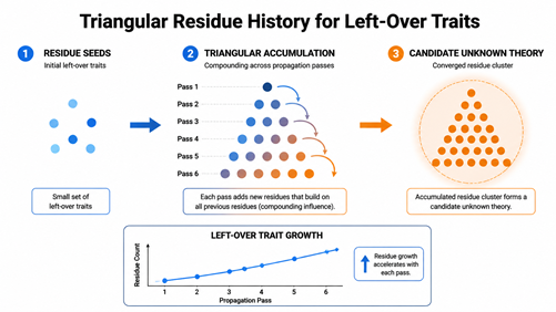
- figure. Left-over Residues, Triangular Residue Theory
- figure. Theory on Triangular Residues
- Screenshots
- Math Theorems
- Wiki Table. Proposed Logic Notation for Pseudocode
- Wiki Table. Token Logic Details in Model
- Wiki Table. How Model Tokens Compare to Linguistics Sememes
- Wiki Table. Current Thermodynamics Research linked to D. and Marletto Principles
- Wiki Table. Comparison of Simple 2-Pass System versus Commercial LLM Model
- Wiki Table. Comparison if Energy Conserved or not in Frameworks
- Wiki Table. Comparison if Matter Conserved or not in Frameworks
- Wiki Table. Is Time Conserved in Frameworks?
- Wiki Table. How to Compare Probability Vector Solutions with Different Lengths & Sequences
- Wiki Table. How LLMs generate Linked Conclusions + Forward Links
- Wiki Table. Simple Reference Table on Common Cosine Similarities
- Wiki Table. Hints on Marletto Style Counterfactual Word Problems
- Wiki Table. Better Coding Routes for Marletto Counterfactuals, ... and Analogies
- Appendix Code
- 1. Expanded Toy for Demo
- Experimenting Draft
- Trial Test Word Problem and Experimental Code
- Testcase 1. for Fire Warning
- Testing Extended deck, mini LLM reasoning
- Result in Wiki Tables from Active State
- Output DFT on Inference Vectors
- Expected Sensitivity from Counterfactual Propagation, Testcase #1
- DFT Residuals - Conclusion concl_damage - Linear
- Draft Figures
- Hidden Comments Section
- Program Change Log
Index for Snippets Concepts DFT on Inference Vectors
Preface
gold 5/16/2026. These are snippets for DFT on Inference Vectors. The model is intended as an exploratory framework for TCL coding. Adding references to Dr. Chiara Marletto's counterfactual framework from the book "The Science of Can and Can't" along with other perspectives. We are using modular snippets inside modular structured programs.
gold 5/16/2026. Upon review of draft page, First Advisor is recommending Discrete Fourier Transform DFT for one, two, or more alternative solutions. In theory, these core axioms, contrast axioms, and Marletto counterfactual axioms as probability vector waveforms could be added and manipulated, and then DFT'ed into multiple solutions vectors. Second Advisor sends feedback for Vector distance along Marletto alternate math calculation pathways: Treat Marletto possible and impossible counterfactuals as multiple vectors in multi-dimensional axiom space and compute cosine similarity and/or phase separation.
I do not have all the answers. The Ideas Seemed to work, but maybe drawbacks? When measured by the Tcl timing statements, completion times and solutions of parameters will differ on different computer set-ups. Assume a future maintainer, either AI Model or human programmer, would have to maintain code with info content and explanatory variable name in program, ref "Snippets Concepts Effects". The Nassi Shneiderman Diagrams NSD or psuedocode Flowcharts pertain to the Tool Control Language TCL computer language as well as other computer languages like Python 3, pseudocode, word logic problems, and technical reports.
For each logic condition selecting a path or calculation task, we might have one, two, or multiple deterministic branches. Attempting to adapt format to multiple probabilistic branches used in Artificial Intelligence AI Models. Then we may use the >>> lottery algorithm <<< to select the winning pathways or tickets.
The existing program has some dummy subroutines. A full construction seems too complex here. I found a paper with images of quantum walks, and I’m wondering if it’s possible to simulate the curves shown in the charts. My advisor has suggested that quantum entanglement/superposition could simulate or underlie quantum worlds, but I’m not sure that I agree. I have limited space on the wiki page, and the fill‑in for the dummy routines has to be pretty brief. In engineering terms, I’m aiming for a “90% solution”, meaning about 90% right and 10% off. Like the simple college formula for a pendulum that is not the exact time series. Call it “fake it ’til you make it” as a college try, but for Quantum Many Worlds. Who is to say? Perhaps you know, TcL specializes in GUI solutions. Maybe try and adapt some starter TcL code for a "quantum worlds slide rule ". Hopefully compatible with the hard-wired classical theory.
Limitations on Tool and Disclaimer
The TCL Snippets illustrate ideal mathematical behavior only and do not perform full simulation, actual measurements, or state vector evolution. The tool only visualizes ideal math structure, whereas no state vector simulation, probabilities, or actual measurement outcomes are derived. This tool for visualization does not simulate actual measurement outcomes or state vector evolution during operations. These are idealized protocols for tutorial purposes. Primarily, TCL /TK uses its strong points here for book keeping and displays. The example tool is not a full emulator. Meaning, limited scope for tutorial purposes.
Disclaimer. None of the computer programs, numerical experiments, power-law fits, or physical analogies described here give a strict, formal proof of the Conjectures, either individually or in combination. The tools and analogies are heuristic models and visualization tools that follow engineering “rules of thumb.” Whereas, pure mathematics has its own shop rules for what counts as a rigorous proof. Any opinions on the difficulty or plausibility reflect current understanding here and programming of the Conjectures as a very hard open problem, not a completed exact math proof, and are offered with full respect for the standards of professional mathematicians.
Extra Significant Figures, If Any in Debugging
In debugging the calculations, some of the printout values reflect roughly 17-digit precision output from a typical double-precision computation. It's not "true exact" beyond 5 significant figures. Extra significant figures are used to check the calculations from other computer set-ups, not necessarily to infer accuracy of data measurements here. Typically, the slight differences in decimal places on far right of decimal point are normal floating-point behavior in Tcl's expr.
Introduction
gold 6/27/2026. Inspired by counterfactual principles discussed in papers and books from Dr. David Deutsch and Dr. Chiara Marletto, see references. With the new logic of Marletto counterfactuals, then the program weighs in counterfactual statement(s) at different ratings of probability. There are possibly both positive and negative counterfactuals. Effectively, the counterfactual axioms are treated as balancing statement(s). For example, a single positive counterfactual might change the overall decision weight from no to yes. The inference engine gains a fresh extension, if the new axioms capture Marletto-style counterfactuals. For instance, a counterfactual axiom stating that possible transformations might be weighted more effectively than static descriptions.
An initial set of Marletto Counterfactual Axioms as states update, amplify, and evolve through local rules, Triangular, and Fibonacci weighting. A Counterfactual Convergence Block has been added for tracking the history of unexpected results. Probabilistic cellular automata PCA is effectively shuffling or reshuffling the hands and axiom scores of the 3 Quantum players. If the Marletto Counterfactual Axioms are treated as inference vectors or signals, then we may apply analogies of Signal Processing to the Counterfactual interplay of ideas. The Triangular and Fibonacci weighting are effectively a form of amplification in Signals Processing terms. Further, the Marletto Counterfactual axioms as vector signals may be analyzed with Discrete Fourier Transforms DFT for both amplitude and phase information.
The program does not calculate real quantum laws. Rather, the program only explores how different weightings on an initial set of axioms and later added counterfactual axioms change the reasoning outcome. From the example axioms tested in the TCL program, we are seeing unexpected amplification or implied importance of "damage." in the fire reports problem. Maybe it was the program set up on the Marletto Counterfactuals, if biased I mean, but there is very little overt mention of damage in the initial fire reports. Classical physics tells us why damage adds up over time. The Quantum-style limits explain why the damage cannot be reversed. As an opinion or corollary, Quantum rules show us why you can not turn back the clock on time. Both sides matter. The program has shown me a new perspective on programming for the Quantum problem, and that is what this Quantum player needed. If not for me, then for other students of Quantum implications.
Note. The term Marletto Counterfactual refers to the nuanced definitions from the recent Marletto papers. There may be differences in evolving definitions from other previous or contemporary writers.
Idea Buster from Solutions out of the Box
Can you define 'solutions out of the box'? Looking for fresh ideas, but getting circular arguments and mirror imaging ideas, as some call it.
There was an ‘idea buster’ that I heard about. Remove one axiom from a set of axioms. This forces a different setup of the problem. It was said that Einstein used this 'idea buster to derive E = mc².
Sometimes theories may emerge by removing a previous or presumed constraint. Then the reduced or current theory is testing what logic structure remains consistent and if producing reasonable parameters. In other words, some theories might be overconstrained in the first place. In that sense, counterfactual reasoning does not merely decorate a theory. The Marletto counterfactual reasoning can redefine the space of allowed explanations. With the changing up or down on the internal program weights and variable weights on the Maletto counterfactual axioms and variables, we are able to shift the inference on the supporting token-like probabilities, support scores, inference weights, and the final decision.
Historical Precedence for Idea Busters
A simple example is the removal of absolute time from Newtonian mechanics. Before relativity, absolute time seemed necessary. Isaac Newton’s formulation in the Principia (1687) treated time as a universal background parameter. In the early twentieth century, Albert Einstein’s 1905 special relativity showed that absolute time was not a fact of nature. Absolute time was a special assumption tied to Newton’s framework. Once that assumption was dropped, time became relative to the observer’s motion. That is an excellent example of a theory changing because one assumption was busted.
Note. Absolute time was an unwritten assumption held by Newton and some contemporaries. Content here is not to imply shedding assumptions or previous misconceptions is easy. Building and proving a new theory from scratch is not a light chore for anyone.
A good example is Modern non‑Euclidean geometry. For centuries, Euclidean geometry was treated as the obvious framework for space, circa 300 BCE . In the nineteenth century, mathematicians like Nikolai Lobachevsky (1829), János Bolyai (1832), and later Bernhard Riemann (1854) showed that non‑Euclidean geometries were fully consistent. Once the parallel postulate or axiom was altered or rejected. That was an “idea buster” in spirit, because removing a single axiom opened an entirely new space of possible theories.
Details. By around 1813, Gauss had developed what he first called anti‑Euclidean geometry. A name he later changed to astral geometry. In a letter written in 1817 to the astronomer Heinrich Wilhelm Matthäus Olbers, Gauss stated his conviction that the physical necessity of Euclidean geometry could not be proven by human reason. This was a striking claim for a working scientist to make about the geometry. Everyone assumed that the Axioms of Euclidean geometry must describe correctly physical space. Gauss never published these results during his lifetime. Later from extant private correspondence, Gauss explained his fear of “the clamor of the Boeotians.” Boeotians was ancient Greek term for Philistines or people hostile to unfamiliar ideas.
Details. Nikolai Lobachevsky, a Russian mathematician, published the first public account of a fully self‑consistent non‑Euclidean geometry in 1829. But the account was in a Russian academic journal with limited circulation outside Russia. János Bolyai published an independent and essentially equivalent result in 1832. János Bolyai, a Hungarian mathematician and the son of Gauss’s friend Wolfgang Bolyai. The new system was included as an appendix to a textbook written by his father. Both mathematicians achieved this result by removing Euclid’s fifth postulate and replacing it with its logical opposite. The assumption that more than one parallel line could be drawn through a given point relative to a given line. The substitution of the negated postulate for the original. The substitution removing one axiom and inserting its negation. This generated an entire new geometry that was every bit as logically consistent as Euclid’s original system. However, the new geometry described curved rather than flat space.
Set theory and algebra also contributed examples. Mathematicians repeatedly found that changing definitions could reveal hidden structure. In the late nineteenth century, there are such mathematicians as Georg Cantor (1874–1897) in set theory and Richard Dedekind (1871–1894) in algebra. They showed that familiar operations could be understood more deeply once the underlying axioms were made explicit. A familiar example is the shift from arithmetic formulas to abstract algebraic rules. This transition was shaped by Dedekind. And later Emmy Noether built on nineteenth‑century foundations, circa 1910. A familiar operation could be studied not only by what the operation computes. But the studies shifted to the axioms that define the operation. Or in some cases, the axioms that un-define or reshape the older proposition into a new idea. That move made mathematics more general and more powerful.
History shows many cases where removing an assumption opened a deeper theory. Before 1900, mathematics, philosophy, and physics all supplied examples of that pattern. The phrases "idea buster" and “solutions out of the box” are therefore fair modern labels for much older practices. Idea busting is the disciplined removal or revision of a hidden constraint so that a theory can be tested at a deeper level. Before 1900, that practice already shaped geometry, mechanics, and philosophy.
This may be a misreading of the Marletto lectures. But in my opinion, some of the math scientists are taking a set of axioms and dropping one or two Axioms to get a “relativity” or "Quantum" solution. You may disagree, but it occurs to me that effectively Dr. Marletto could block some axioms in a set of axioms with these counterfactuals. I think this TCL code deck could be set up to selectively block a set of axioms. But you can tell me different.
Counterfactual Model Testing
Counterfactual axioms push theories to show their real strength. They force you to figure out which parts of your model actually explain things, and which parts you’re just repeating out of habit. If your model only works when you never touch the familiar assumptions. Chances are it depends on unnecessary constraints you haven’t noticed. Start flipping one rule at a time and see what holds up. That’s how you sort the essential ideas from the baggage.
Counterfactual model testing takes this mindset and gives it some discipline. It’s not just about whether your model fits the data we already know. It’s about asking, “What if this assumption changed?” Maybe you delete the assumption, maybe you reverse the assumption. Whatever gets the gears turning. You’re not trying to describe reality perfectly here. The goal is to stress-test the logic, break the model out of its comfortable mold, and maybe find new explanations. So you can think of counterfactuals almost like intellectual crowbars. Counterfactuals pry open the standard picture and show you what else might be possible.
This kind of challenge matters. Lots of theories seem airtight until you knock out one hidden pillar. A good model shouldn’t just limp along in its favorite setup. A good model should make clear why that arrangement is special, and what falls apart (or gets stronger) when things shift. That’s how counterfactual axioms sharpen fuzzy ideas, testing the structure, consistency, and the real depth of our explanations.
What Einstein actually did?
It’s funny when you think about it. Early twentieth-century German physics actually grew out of a cultural scene shaped by Hegel, Schelling, and neo-Kantianism. The history of physics isn’t just about experiments and math. History includes the ideas that people bring into the lab, too. In this case, those ideas came straight from the heart of German philosophy. Einstein rejected Hegel’s metaphysics outright, but Einstein did pick up on the Hegelian idea that you can rebuild a theory by shifting its core assumptions. That’s a real influence, just not a mystical one.
What Einstein actually did was simpler and sharper. Einstein took out hidden starting points in a theory and rebuilt it based on whatever stayed unchanged. In special relativity Einstein threw out absolute time. But Einstein kept the speed of light as something that can’t budge. In general relativity, Einstein dumped the idea of gravity as a force and reframed it as the geometry of spacetime. For the developments that led to the equation E = mc², Einstein dropped the old split between mass and energy as separate conserved things. His 1905 paper just imagined a body sending out two pulses of light—momentum conservation and the Lorentz transformations do the rest. Einstein proved the body loses mass in direct proportion to the released energy divided by c². There’s no dialectic here, just rigor and math and the logic of constraints.
Simple Reduction Protocol
- Remove an assumed constraint or axiom.
- Check what remains logically consistent.
- See whether the reduced system explains more or less.
- Treat the reduced system as a hypothesis.
Simple Analogies for Marletto Counterfactual Protocol
Think of a man walking a long road of mud puddles on swampy ground. He is thankful for several intervals along the road of solid ground called islands or axioms of truth. But He carries several long counterfactual planks to line his path across the mud puddles. The man is very forgetful of where he leaves his planks or bridges between truths. But if he pulls up the planks behind him, his original path into the swamp, and even out of the swamp, may not be reversible.
Spelled out section. A classical view only maps the path on the swampy road that was actually taken. A Marletto viewpoint maps crossings were genuinely possible and which were not possible, with the tracks of the counterfactuals.
Treat like a scale that weighs pennies as arguments. The right scale is for pennies as the main set of positive axioms. The left scale is for pennies as contrast arguments. When the scale is pointing right or left of the center mark, a counterfactual penny or more is tossed L&R to counter weigh the conventional physics.
Spelled out section. The scale does not ask only what was seen as final result. A Marletto viewpoint asks what would still be possible if the L&R scales were prepared in a different way.
Word Problems in Marletto Counterfactual Style
I use simple word problems or models as preparation for coding. The following counterfactual examples were developed for TCL coding. The worked problems or models draw inspiration from the constructor theory framework of Dr. David Deutsch and Dr. Chiara Marletto.
1. Coffee Cup
- Possible Task: Heat flows from hot to cold.
- Impossible Task: Coffee reheats itself from room temperature.
- Solution Hint: 2nd law of thermodynamics forbids spontaneous heat flow from cold to hot.
2. Mixing Dye in Water
- Possible Task: Dye spreads naturally in water.
- Impossible Task: Dye unmixes by itself back into a drop.
- Solution Hint: Entropy always increases — it doesn’t decrease on its own.
3. Document Copy
- Possible Task: A copier duplicates text from paper.
- Impossible Task: Perfect copy of an unknown quantum state.
- Solution Hint: No-cloning theorem blocks perfect quantum copying.
4. Broken Glass
- Possible Task: Glass shatters when it hits the floor.
- Impossible Task: Glass reassembles itself from the pieces.
- Solution Hint: Entropy rise makes that kind of reversal basically impossible.
5. Plant Growth
- Possible Task: Seed grows into a full plant.
- Impossible Task: Plant shrinks back into a seed.
- Solution Hint: Life needs steady energy input to grow and stay organized.
6. Battery Discharge
- Possible Task: Battery slowly loses its charge.
- Impossible Task: Battery charges itself without any help.
- Solution Hint: Energy naturally flows from high potential to low.
7. Information Erase
- Possible Task: Delete a file from the drive.
- Impossible Task: Erase information with zero trace.
- Solution Hint: Landauer’s principle says erasing always requires some energy.
8. Ball Rolling
- Possible Task: Ball rolls downhill.
- Impossible Task: Ball rolls uphill all by itself.
- Solution Hint: Gravity pulls it down, needs extra force to make it rise.
9. Ice Melting
- Possible Task: Ice melts in a warm environment.
- Impossible Task: Ice forms by itself in heat.
- Solution Hint: Heat melts ice, it doesn’t freeze it again.
10. Paper Burn
- Possible Task: Paper burns and turns into ash.
- Impossible Task: Ash turns back into paper.
- Solution Hint: Combustion is an irreversible chemical change.
11. Light Switch
- Possible Task: Flipping the switch turns the light on.
- Impossible Task: Light turns on just by thinking about it.
- Solution Hint: Needs real physical action, not pure mind power.
12. Password Check
- Possible Task: Verify a known password.
- Impossible Task: Guess an unknown password instantly.
- Solution Hint: Brute force still takes time and lots of attempts.
13. Fire Alarm Delay
- Possible Task: Smoke triggers the alarm early.
- Impossible Task: Alarm only triggers after full burn.
- Solution Hint: Early detection can prevent a lot of major loss.
14. Hidden Damage Buildup
- Possible Task: Small damage grows over time.
- Impossible Task: Damage shrinks by itself.
- Solution Hint: Once it crosses the threshold, it’s usually irreversible.
15. Late Fire Report
- Possible Task: Report sees visible flames.
- Impossible Task: Report somehow undoes past damage.
- Solution Hint: Damage keeps accumulating and can’t be reversed.
16. Missed Early Signs
- Possible Task: Detect smoke at low level.
- Impossible Task: Ignore smoke and assume no damage will happen.
- Solution Hint: Small signs often lead to big losses if ignored.
17. Irreversible Fire Spread
- Possible Task: Fire spreads from a single spark.
- Impossible Task: Fire returns to cold ash on its own.
- Solution Hint: Entropy drives destruction in one direction only.
18. Cumulative Heat Damage
- Possible Task: Heat builds up slowly.
- Impossible Task: Heat dissipates without any help.
- Solution Hint: Late response usually means total loss.
19. Fire Report Weighting
- Possible Task: Weight "smoke" reports higher.
- Impossible Task: Weight only "flames" reports.
- Solution Hint: Early signals beat late ones most of the time.
20. Generic Report
- Possible Task: True = 1
- Impossible Task: Not True = 0
- Solution Hint: A contradiction. I am stumped, unless both are true in Quantum Logic?
Note. Somehow, I develop a movie in the mind that shows the described possible actions, and then the impossible actions play out. But I guess that Dr. Marletto would tell me the rewind button of backward time is forbidden to me. As irreversible damage has occurred in the movie of my mind. This rewind button should be like the "-time" ,"restart", "clear", or "reinitialize" buttons in some of my TCL calculators.
Possible Coding Extensions to Token-like Mini-LLM Reasoning
Fourier Analysis on Multiple Solutions in Triangular Vector Form
Finally, if you run a Discrete Fourier Transform (DFT) on a triangular-weighted probability vector, you’ll pick up:
- "Direct Current" levels
- Strong low-frequency parts — the overall dominant messages.
- Odd mid-frequency bumps, where all that accumulation creates “beats” or resonant patterns between what’s possible and impossible.
- Sharp high-frequency peaks, flagging those “Left-Over” traits — the tenacious minority bits that just won’t get crushed by the bulk.
Note. The present Nomenclature for Discrete Fourier Transform (DFT) etc was derived from the Electrical Engineering profession and may not match up, too well with the Marletto/Quantum terms.
Second Advisor sends feedback for Vector distance along Marletto alternate math calculation pathways: Treat Marletto possible and impossible counterfactuals as two [ or more ... ed. ] vectors in multi-dimensional axiom space and compute cosine similarity and/or phase separation.
For two vectors, we can estimate the angles between and effectively the difference between the solution vectors in solution space.
What does the Fourier Program really do?
When you use Fourier transforms with rule systems, you get a new angle. Typical probability just bumps single numbers up or down. But the Fourier transform exposes how your whole set of results might have underlying “rhythms.” Think about listening to a musical chord: the main signal loudness comes from the DC component. Everything else shapes the mood—smooth, tense, or somewhere in between.
What does the program really do? First, the program reads the inference rule scores like a frequency pattern. Then it uses the Fourier transform to break down what’s positive, negative, or left over. For some inference vectors, this even helps make sense of how tightly chunks of information clump together.
The most important Fourier term is the zero-frequency part and shows overall support. The smaller, higher-frequency pieces show how support rises and falls as you step through the list of rules. In a vector’s Fourier transform, each frequency component has a phase (where in its cycle it starts) and a magnitude (how strong it is). Magnitude is the “volume” of that frequency. Phase is the timing.
If two sine waves match in frequency and amplitude, but one’s a little delayed. That’s what “phase” is. Don’t think of phase as noise. It’s crucial information. Phase tells your transform how to rebuild the original pattern in the right shape.
Mathematically, for a vector with real numbers, the DFT gives you complex numbers. The length or absolute value is the magnitude. The angle or argument is phase. When magnitude is big and phase lines up well, you’ve got a key frequency in your pattern. If the magnitude is zero, phase drops out and doesn’t matter.
Why does this matter? Magnitude tells you what’s in the pattern, but phase tells you how those pieces fit together. Two vectors can have identical magnitudes and still look way different if their phase arrangements shift.
Bringing this back to your set of inference vectors or rules. Each list of confidence values for various statements is treated as a signal. This is not a sound wave. Just numbers showing a set of rules or ideas that are either how strongly consistent or inconsistent.
Note. Each vector number represents confidence in one inference rule. We treat the entire list of rules as a short discrete signal. Low frequency components will show broad consensus. High frequency components will show sharp differences.
Initial Problem Statement, but Program much adapted from this
Program consists of a sequence of weighted decisions that vote on a yes-no decision. Suppose one first comes up with a no decision weighted at 49% yes, 51% no. With the new logic of counterfactuals, then the program weighs in counterfactual statement(s) at probability of 0.75. There are possibly both positive and negative counterfactuals. Effectively a balancing statement(s), the positive counterfactual changes the decision weight from no to yes. The inference engine gains a fresh extension, if new axioms capture Marletto-style counterfactuals. For instance, a counterfactual axiom stating that possible transformations might be weighted more effectively than static descriptions. The negative counterfactual votes and may change the decision weight from yes to no.
The program does not calculate real quantum laws. It only explores how different weightings on an initial set of axioms and later added counterfactual axioms change the reasoning outcome.
A Fresh Unified Theory Probably Won't ...
A fresh unified theory probably won’t come from just picking sides of two arguments in physics, particle or wave. But from digging into the messy bits both theories leave behind. These leftover signals that show up strongly in both positive and negative zones. Leftover Signals are the paradoxes our current theories just can’t handle well. This is where Constructor Theory shines, since Constructor Theory is built to zero in on what’s actually possible and impossible. The comparison of solution vectors takes this idea and gives it teeth. Constructor Theory highlights exactly where classical assumptions crack, where quantum reversibility collapses under gravity, and where something like energy conservation ties different domains together. Then there’s triangular propagation. Triangular propagation works like a spotlight, making these tensions stand out and stick around.
This whole process acts like an “idea buster” in code. Pull away the assumptions, see what still fits, and suddenly you can spot the gaps.Those awkward places where current ideas fall short and you need new rules. The engine even reveals that the way information moves can be just as important as the info itself. Try out different weighting styles—linear, triangular, Fibonacci. Each weighting style brings different hidden leftovers into focus.
Now, if you run a Discrete Fourier Transform (DFT) on a probability vector that’s been weighted with a triangular factors, you’ll notice a few things:
- Strong low-frequency pieces that stand for big-picture, dominant conclusions.
- Mid-frequency spikes where patterns overlap, creating beats or resonances where possible and impossible collide.
- High-frequency blips that point out sharp conflicts, the stubborn minority cases that just won’t blend in.
Switching to this frequency perspective of Fourier transforms often uncovers tensions. Meaning tensions that you’d miss if you only stuck with straight linear scoring or even triangular methods. Fourier transforms shine a light on the details of vector solutions hiding in plain sight.
Note. The DC component (k=0) is the most important single number in DFT analysis for the probability vectors. The DC component represents the average magnitude (total "energy" or overall confidence) of the entire vector.
Grounds for Further Extensions
If you think of a theory as a collection of constraints, then deleting a constraint is a controlled experiment. You’re watching how the counterfactual scaffolding reshapes itself when you kick out one of its supports. That’s pretty much how Einstein worked. Einstein would discard an assumption that blocked him from seeing new invariants. Then Einstein would figure out what still held up. In this system of inference vectors, pulling an axiom has a clear effect. The pattern of inference vectors shifts, the way information propagates in the triangular scheme changes, and the DFT spectrum warps. The “sound” of the probability distribution changes. How much it warps tells you a lot. If the results stay well‑behaved, the theory was probably overloaded with requirements. If everything goes wild, that dropped axiom really mattered. This trick gives you a direct handle on which parts of a theory are foundational and which are historical clutter.
You can push or extend this by hunting for the invariant core of a theory. The core or backbone that endures no matter what constraint you poke at. Sometimes, no matter how you tweak the weights, some features of the inference vector remain untouched. These are your real anchors. In Constructor Theory language, these are the tasks always possible, regardless of how you set up the rest. In Fourier-speak, these show up as stable, low-frequency modes that survive after the rest of the structure shifts around. Laying out these “deep” invariants cuts through superficial agreement between different theories and shows where frameworks are genuinely talking about the same thing.
There is also much traction in using the DFT tools that you already have on the wiki. When you add or remove axioms, the DFT signature tells you a lot about how the inference engine is reorganizing. A smooth spectrum means the theory is internally consistent. Jagged, jumpy lines point to places where things don’t fit, or you’re dragging around unnecessary leftovers. This frequency‑domain look complements basic probability scores. The Fourier transform gives you a second, more visual window into what the logic engine is actually doing.
A further leap is mapping all of this onto Constructor Theory. Every axiom carves up the world into what’s possible and what’s not. Remove an axiom and you redraw the lines around feasible tasks. The current inference engine is already keeping track of these shifts. The inference engine sorts which counterfactuals survive, which get blocked, and which pile up as “leftovers.” Formalizing these zone shifts means you can see directly how different sets of starting facts partition up the same space of explanations. You stop thinking just in terms of equations, and start thinking in terms of shifting “possibility frontiers,” which is exactly Constructor Theory’s game.
You’ve also got room to dig deeper into how classical and quantum inference react when you start pulling structural supports. The triangular propagation approach already produces vectors that act Newtonian, quantum-like, and “third channel” leftovers. When you relax constraints, each of these rule systems or inference vectors behaves differently. And, weirdly, the residues sometimes operate in spectral bands untouched by the classic or quantum channels. Laying these responses side by side could clarify when quantum structure emerges, when classical structure falls apart, and when something irreversible shows up.
All this connects cleanly to Einstein’s actual historical method. Einstein treated theory as a kind of axiom surgery: Remove “absolute time,” see what’s left. Remove “gravity as a force,” see what emerges. Remove “mass and energy are separate,” see what structures hold. Retelling the results of your code and DFT plots as a kind of modern replay of Einstein’s sequence or protocol. Both inference vectors and Fourier transforms grounds the mathematics for the humanities crowd and makes the method feel less esoteric or mystical. It’s just disciplined logic. This is the bridge that links counterfactual reasoning with both mathematical form and historical precedent.
Second Advisor sends feedback. The next step is to treat Axiom Removal as a Formal Operator. Define an operator A⁻ that acts on a theory T to produce a reduced theory T′. Then study the stability of inference vectors under A⁻. T' = A⁻(T) This becomes a new kind of “differential geometry of theories.” Where the curvature measures how violently the inference space reorganizes when a constraint is removed. That is a mathematically clean way.
Possible Coding Extensions to Token-like Mini-LLM Reasoning
The Extension now saves every run. The program records both the softmax probability table and the wiki table with a timestamped filename. Every session gets logged. Nothing gets lost or overwritten. The main improvements here are simple but useful. The program writes every result to tape/file. There are timestamps used in filenames to keep all runs separate from overwrite.
Normalize Ordering Upfront. Developed code is heavily dependent of the order of Axioms. Define a canonical ordering rule once and stick to it. Much more theory and unforeseen impacts to results on this order of axioms, but probably a major concern in code.
Examples:
- Order by logical dependency (foundational concepts first).
- Order by historical appearance in the development of the theory.
- Order by decreasing confidence score (strongest beliefs first, max Bayesian prob. ).
- Order by multiple random sequences of axioms. My preference
     and this would offer max. prob. of multiple solutions to LLM coding.
     But difficult "sell" to engrs
     used to deterministic single solutions.
Note. Multiple Random Sequences refers to easy ensemble averaging.
Note. Recommendation: Use "Logical Dependency" for primary run. Add "Multiple Random" ensemble to quantify ordering sensitivity Report both main result and variance band.
Later Feedback from Second Advisor
gold Update and paraphrased from Second Advisor, 6/25/2026. Probabilistic cellular automata is closer code architecture, as currently laid out. Code architecture in prototype has not conventional Bayesian features. Code is Exploratory inference engine based, stochastic rules and spectral analysis. Seems possible to recast features for better convergence on results, but save what DFT utilities has been gained so far. Core model would be Probabilistic cellular automaton on axiom weights w/ counterfactual groups.
gold Updated 6/27/2026. Thank you for your suggestions. The new program is working very close to expectations. Meaning, no grand conclusions were expected on Quantum rules, but I wanted a new look or gander at the elements or axioms of the Marletto counterfactuals involved in the Quantum rules. Probabilistic cellular automata PCA is effectively shuffling or reshuffling the hands and axiom scores of the 3 Quantum players. The program has shown me a new perspective on the Quantum problem, and that is what I needed. If not for me, then for other students of Quantum implications.
The program was written with modules and as generic variables as possible. The example is showing an unexpected rise or amp in the "damage" axiom from the initial conditions before the "fire alarm" starts. That is, under Quantum rules, "damage" can not be reversed is a major factor for the discussion.
Summary
Constructor Theory protocols are little radical to brains trained on Newtonian. In opinion here, do not expect solution(s) involving counterfactuals to be familiar deterministic algorithms with a single solution.
So, seeing things through the Fourier frequency lens reveals tensions and leftovers you wouldn’t spot just by stacking or scoring everything the usual way. This inference engine doesn’t just process evidence. The inference engine digs in the cracks, pulls up the floorboards, and shows you what’s still hiding underneath.
As comparison to programming in deterministic logic from the 1970's Fortran 77 and 1990's TCL. These Linked Conclusions and associated Forward Links in the program over the probabilistic data tokens are perhaps the nearest equivalent to the deterministic logic and Galileo / Newtonian variable type laws, that one will see in the deck.
The example tool and discussion here is not a full emulator of the massive LLM Models. Meaning, limited scope and much granularity in the probabilistic reasoning for tutorial purposes.
References
- Snippets Concepts DFT on Inference Vectors
- Snippets Concepts Triangular Propagation
- Snippets Concepts Inference Engine
- Snippets Concepts Diósi Penrose Model
- Snippets Concepts Quantum Fourier Transform
- Snippets Concepts Lottery Pruning
- Snippets Concepts Qubits Model
- Snippets Concepts Collatz Plotter
- Snippets Concepts Geometric Tunneling
- Snippets Concepts Collatz T-Stop
- Snippets Concepts Random Cubics
- Snippets Concepts McCarthy 91_Function
- Snippets Concepts Predator Prey
- Snippets Concepts Thomas Solver
- Snippets Concepts Grover Simulation
- Snippets Concepts Radioactive Decay
- Snippets Concepts Hypersphere Simulation
- Snippets Concepts Nassi Shneiderman Flowcharts
- Snippets Concepts SlideRule to Quantum
- Snippets Physics Concepts Qubits
- Snippets Physics Concepts Feynman
- Snippets Physics Concepts Quantum
- Snippets Physics Concepts Toy
- Snippets Physics Concepts Minimalism
- Zero Handling Workarounds
Note. These Snippets on Theoretical Physics are a set, not stand alones. Recommend read all of the set.
- A little slide-rule on TCL Wiki, ( much credit for the algorithms in the sliderule. )
- Richard Suchenwirth 2003-08-31
- Smoothing and differentiation of data by simplified least squares procedures
- Savitzky, A. ; Golay, M. J. E. Two examples are presented as subroutines in the FORTRAN language.
- Savitzky Golay Filtering, Python
- Savitzky Golay Filtering — SciPy Cookbook documentation
- Smoothing Example with Savitzky-Golay Filter in Python
- Introduction to the Savitzky-Golay Filter: A Comprehensive Guide (Using Python), Thomas Konstantinovsky
- Konstantinovsky has good explanation. Note detailed. WhittakerSmoother in Python
- The Perfect Way to Smooth Your Noisy Data, Whittaker-Eilers smoother, Andrew Bowell
- Feb 28, 2024
- A Basis for a Mathematical Theory of Computation,Author(s)
- McCarthy, John
- John McCarthy: A basis for a mathematical theory of computation, in:
- Computer Programming and Formal Systems.
- P.Braffort, D.Hirschberg (ed.), Amsterdam:North Holland 1963,
- several versions, archived pdf
- McCarthy’s LISP and Basis for Theory of Computation, archived pdf
- en.wikipedia.org search on <John McCarthy computer>
- John McCarthy at Stanford web site, archived
- Towards a Mathematical Science of Computation, J. McCarthy,
- Computer Science Department, Stanford University, archived pdf
- Elephant 2000: A Programming Language Based on Speech Acts
- John McCarthy, Stanford University, archived
- Elephant input and output statements are characterized
- as speech acts and programs, which
- can refer directly to the past.
- Elephant proposal contains summary
- on McCarthy mathematical theory of computation
- Mysteries and other Matters, development of Lisp , archived
- Note. A lot of early papers and notes from John McCarthy and Knuth are difficult to assess web links or archived.
- Machine Learning Approaches to the Collatz Conjecture:
- A Comprehensive Framework for Pattern Recognition
- and Automated Conjecture Generation. IJIRT, Vol. 12 Issue 7
- Transformers Know More Than They Can Tell:
- Learning the Collatz Sequence , arXiv:2511.10811
- The Collatz conjecture, Littlewood-Offord theory, and powers of 2 and 3,
- Aug 2011, Terence Tao,
- mentions Gambler's Ruin on this 2011 post, but better search on his website for updates.
- Efficient Computation of Collatz Sequence
- Stopping Times: A Novel Algorithmic Approach ( credit for the new algorithm. )
- EYOB SOLOMON GETACHEW, BEAKAL GIZACHEW ASSEFA
- The Collatz Conjecture over the Gaussian Integers, Alejandra Alvarado
- An example of the difference between quantum and classical random walks
- Andrew M. Childs, Edward Farhi, Sam Gutmann ( much credit for the new algorithm. )
- Simple Program Design, Lesley Anne Robertson, 2004
- Lecture in Spanish, diagrama de nassi schneiderman o rectángular
- website for estudia con nancho, 2023
- Lecture, Communicating Complex Logic with Ease
- with Nassi-Shneiderman Diagrams, Atanas Marchev,
- Jetbrains MPS community, 2023
- Java library for working with Nassi-Shneiderman diagrams
- (structograms) from Atanas Marchev, Github website
- Flowchart techniques for structured programming
- Authors: I. Nassi, B. Shneiderman, circa 1973
- KernelF- an Embeddable and
- Extensible Functional Language, Markus Voelter
- voelter = acm, ~~ 2023
- Algorithmic Accountability: Designing for Safety , Ben Shneiderman,
- Radcliffe Institute, 2018
- the lottery ticket hypothesis:
- finding sparse, trainable neural networks, jonathan frankle, mit
- 4 mar 2019, michael carbin
- Maria Violaris, arXiv preprint titled "Quantum observers can communicate across multiverse branches." Jan 2026
- Vafa, Cumrun (September 2006). "Baby universes and string theory". International Journal of Modern Physics D. 15 (10): 1581–1586.
- Lecture from Sean Carroll: The many worlds of quantum mechanics
- Lecture from Sean Carroll: Quantum Mechanics and the Many-Worlds Interpretation
- Lecture on many worlds theory, Does Quantum Mechanics Reveal the Secrets of Parallel Universes?
- Emergence of Classicality in Wigner’s Friend Scenarios, Tom Rivlin, Jul 2025
- Quantum Superpositions of Conscious States in a Minimal Integrated Information Model, Kelvin J. McQueen, April 2026
- Wigner's friend scenarios: on what to condition and how to verify the predictions
- Flavio Del Santo, Jul 2024
- A review and analysis of six extended Wigner's friend arguments
- David Schmid, Yìlè Yīng, Matthew Leifer, Aug 2023
- The Many Worlds of Hugh Everett III : Multiple Universes,
- Mutual Assured Destruction, and the Meltdown of a Nuclear Family
- Peter Byrne, 2010
- The Many-Worlds Interpretation of Quantum Mechanics (level 3 multiverse), dissertation,
- Everett, Hugh
- An Undergraduate Course in Quantum Computing, Peter Young, Apr 2026
- # Based on ref. An Undergraduate Course in Quantum Computing, Peter Young, Apr 2026
- # Much credit for the quantum circuit diagrams, Matches textbook Fig 16.4 etc
- # University of California Santa Cruz, CA, arXiv:2604.10396
- Does gravity follow the rules of quantum mechanics? Press Release, Prof. Kazuhiro Yamamoto
- Momentum squeezed state realized via optimal filtering in optomechanics:
- Implications for gravity-induced entanglement”, Ryotaro Fukuzumi, Published 13 April,2026.
- Bose-Marletto-Vedral experiment without observable spacetime superpositions
- Nicetu Tibau Vidal,Chiara Marletto
- The Science of Can and Can't : A Physicist's Journey Through the Land of Counterfactuals
- by Chiara Marletto, 2021.
- Quantum Coins and Counterfactuals, in Consistent Quantum Theory, Robert B. Griffiths, 2002,
- from CMU Quantum Theory Group
- How to Rewrite the Laws of Physics in the Language of Impossibility,
- Amanda Gefter, Contributing Writer, April 29, 2021
- Fundamental properties of beam-splitters in classical and quantum optics: arxiv /abs/2303.13705
- Masud Mansuripur, Ewan M. Wright, 2023
- Constructor theory, Wikipedia, date 4/27/2026
- Constructor theory of probability, 2016,
- Chiara Marletto
- Bernstein, G. A. (2026c). Reality is mathematical structure.
- Bernstein, G. A. (2026e). Why these simple laws?
- Deriving physics from mathematical necessity.
- Bernstein, G. A. (2026h). The arrow of time is irreversible computation.
- Deutsch, D. (2013). Constructor theory. Synthese, 190(18), 4331-4359.
- Deutsch, D., & Marletto, C. (2015). Constructor theory of information. Proceedings of the Royal
- Society A, 471(2174), 20140540.
- Deutsch, D. (1997). The Fabric of Reality. Penguin.
- Deutsch, D. (2011). The Beginning of Infinity. Penguin.
- Marletto, C. (2021). The Science of Can and Can't. Penguin.
- Popper, K. (1972). Objective Knowledge. Oxford University Press.
Note. The ink is hardly dry on some of these papers. Don't know what gems are hidden, if I dig deeper.
Screenshots
figure. Analogy of Scale

figure. Analogy of Turing Machine
Credit to website. Max runs computers by Maxwell Anselm
figure Solar Oven
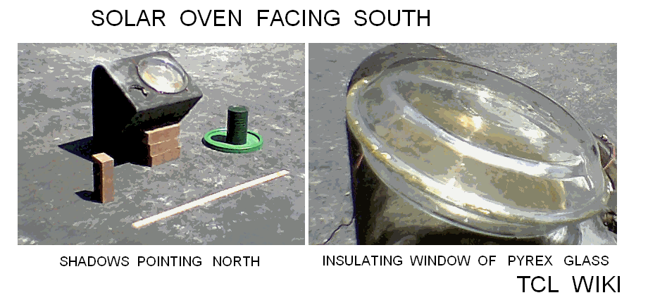
figure Solar Oven 2
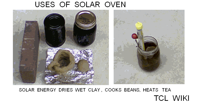
figure Mockup Display on Fire Warning
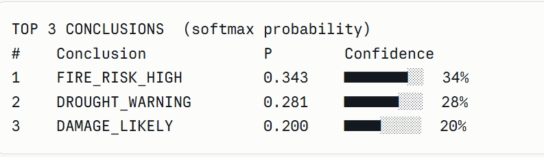
figure. Theory on Triangular Math
figure. Triangular Propagation, Positive Counterfactuals
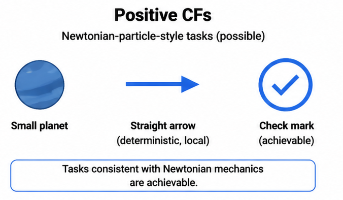
figure. Triangular Propagation, Negative Counterfactuals
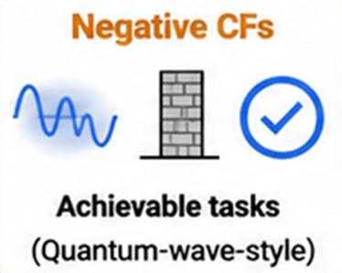
figure. Triangular Propagation, Leftover Counterfactuals from Both Regiemes
figure. Left-over Residues, Triangular Residue Theory
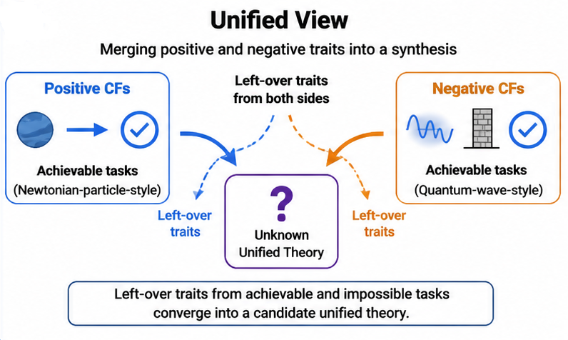
figure. Theory on Triangular Residues
Math Theorems
# ascii, very close to pseudocode needed

T' = A-(T)

an axiom vector

a = (a1, a2, ..., an)

an inference vector

p = (p1, p2, ..., pm)


A-_k(a) = (a1, a2, ..., 0, ..., an)

a new inference vector

p' = F(a')

cosine similarity score:

S_k = (p dot p') / (||p|| * ||p'||)
K_k = 1 - S_k
----
DEMO: AXIOM REMOVAL AS FORMAL OPERATOR A^-

1. Simple Theory Model
----------------------
Let theory T be represented by a set of axioms and their inference consequences.

Example base theory T0 (Fire Risk Domain):

Axioms:
A1: High heat implies increased ignition probability
A2: Dry conditions strengthen spark events
A3: Wind amplifies damage propagation
A4: Spark events cause observable smoke

Inference vector V(T) = [fire_hi, damage, bridge]
                      = [0.82, 0.31, 0.45]   (normalized strengths)

2. Axiom Removal Operator A^-
----------------------------

Definition:
T' = A^-(T, Ai)   removes axiom Ai from T

Effect on inference vector:
V(T') = M_i * V(T)

Where M_i is a reduction matrix for removing axiom i.

Simple 3x3 demo matrices (illustrative):

Remove A1 (heat):
M1 = | 0.6  0.0  0.0 |
     | 0.0  1.0  0.0 |
     | 0.0  0.0  0.9 |

Remove A3 (wind):
M3 = | 1.0  0.0  0.0 |
     | 0.0  0.7  0.0 |
     | 0.0  0.0  0.4 |

3. Demo Calculation
-------------------

Original:   V0 = [0.82, 0.31, 0.45]

After removing heat axiom (A^- on A1):
V1 = M1 * V0 = [0.492, 0.31, 0.405]

After removing wind axiom (A^- on A3):
V3 = M3 * V0 = [0.82, 0.217, 0.18]

Change magnitude (stability measure):
Delta(A1) = ||V1 - V0|| = 0.341
Delta(A3) = ||V3 - V0|| = 0.312

Higher Delta = higher "curvature" when removing that axiom.

4. Differential Geometry Analogy
--------------------------------
Think of theories as points in inference space.
A^- is like a directional derivative.

Curvature K(Ai) ≈ |Delta(V) / strength_of_Ai|

High curvature axioms are "load-bearing"
- removing them violently reorganizes the inference space.

5. DFT on Inference Vectors (Snippet Concepts DFT on Inference Vectors )
---------------------------------------------
Apply Discrete Fourier Transform to sequence of reduced theories:

Let sequence S = [V(T), V(A^-(T,A1)), V(A^-(T,A2)), ...]

DFT reveals dominant "frequencies" of inference change
- i.e. which axiom removals cause low-frequency (stable)
vs high-frequency (chaotic) shifts in conclusions.

Low-frequency components = robust core theory
High-frequency components = brittle, axiom-sensitive parts

Bottom Line:
The operator A^- turns axiom removal into a clean mathematical object.
We can measure how much a theory "bends" when constraints are removed.
This gives a quantitative way to find the minimal stable core of any theory.

This demo uses linear algebra for simplicity.
Real versions could use logic lattices
or vector embeddings of propositions.
Wiki Table. Proposed Logic Notation for Pseudocode
| Index No. # | Concept | What Logic Notation Proposed | What Model Actually Uses Internally | Closeness | Quibble_Notes |
|---|---|---|---|---|---|
| 1 | Form | Prog → Und = 0.95 | High-dimensional vectors + directed attention weights | Very High | Scalar simplified; internals use 1000s of dimensions |
| 2 | Directionality | Token_A → Token_B | Attention flows from query token to key/value tokens | High | Forward influence only — A affects B |
| 3 | Direction Clarification | Prog → Und = Prog activates Understanding | Attention score shows how strongly one token attends to another | High | No reverse gears or reverse thinking; purely forward |
| 4 | Example Token | Prog → Und = 0.95 | Prog embedding strongly activates Understanding features | Very High | "Programming forces understanding" |
| 5 | Example Token | Prog → Prec = 0.92 | Prog vector directs high weight toward Precision | Very High | "Programming demands precision" |
| 6 | Example Token | Prog → Clar = 0.89 | Prog embedding builds Clarity activation | High | "Programming builds clarity" |
| 7 | Example Token | Prog ⊥ Amb = 0.90 | Prog vector strongly suppresses Ambiguity features | High | ⊥ symbol = confronts / rejects ambiguities |
| 8 | Example Token | Prog → Log = 0.85 | Prog embedding imposes and strengthens Logic | High | "Programming imposes logic" |
| 9 | Example Token | Hum → Flaw = 0.80 | Human_Mind embedding activates Flaw-glossing | Medium-High | "Human mind glosses flaws" |
| 10 | Example Token | Paper → Err = 0.75 | Pencil_Paper embedding tolerates Error patterns | Medium-High | "Pencil paper forgives errors" |
| 11 | Weighting | Scalar strength 0.95 | Continuous floating-point attention scores | High | Weights recalculated dynamically per context |
| 12 | Atomic Unit | Compact 3-word SVO token | Dense sub-token embeddings + contextual activations | High | Notation tokens are clean, human-readable versions |
| 13 | Composition | Chaining tokens | Multi-layer transformer composition of representations | High | Massively parallel across many layers & heads |
| 14 | Overall Style | Weighted directed tokens | Attention-weighted semantic feature flow in residual stream | Very High | One of the best intuitive approximations of Model internals |
Note. SVO for {Subject, Verb, Object } order.
Note. Alternate text. Attention mechanisms compute weighted directed connections between every token and every other token: Token_A --weight 0.87--> Token_B . Like the probabilistic shorthand, but binary code with hundreds of dimensions and thousands of parallel "directions" (attention heads).
Notation [Prog → Und] = 0.95 is not really Polish notation.
Polish notation (prefix notation) puts the operator first: + 3 4 or Force Prog Und.
Intermediate form is closer to infix with directed arrow, like a weighted graph edge or a simple assignment.
It is not applicable as true Polish notation.
It is much closer to:
Weighted directed graph notation (A → B [weight])
Attention mechanism style (Token_A --[0.87]--> Token_B)
Wiki Table. Token Logic Details in Model
| # | Concept | What Proposed | What Model Actually Uses Internally | Closeness | Quibble_Notes |
|---|---|---|---|---|---|
| 1 | Form | Prog → Und = 0.95 | High-dimensional vectors with directed attention weights | Very High | Scalar is simplified; internal uses hundreds of dimensions |
| 2 | Directionality | Directed (→) | Strongly directional (attention heads are directed) | High | Attention is multi-headed and bidirectional in practice |
| 3 | Weighting | Scalar probability/strength (0.95) | Continuous floating-point strengths (attention scores) | High | Weights are dynamic and change with context |
| 4 | Atomic unit | Compact token triple | Sub-token embeddings + contextual activations | High | Internal units are much denser than 3-word triples |
| 5 | Composition | Chaining tokens | Transformer layers composing representations | High | Composition is massively parallel across many layers |
Wiki Table. How Model Tokens Compare to Linguistics Sememes
| # | Aspect | Linguistic Sememes | AI Model Tokens / Architecture | Intermediate Notation Axioms | Similarity | TCL Syntax Comparison | Quibble_Notes |
|---|---|---|---|---|---|---|---|
| 1 | Size | Atomic (very small) | High-dimensional vectors (thousands of dims) | Prog → Und = 0.95 | High | TokenStoreDict keys (14-15 chars) | Intermediate is compact human bridge |
| 2 | Function | Basic building blocks of meaning | Activation patterns in residual stream | Prog → Force(Und) | High | dict set TokenStoreDict ... | AI tokens are learned vectors |
| 3 | Structure | Feature bundles +human+adult | Multi-head attention weights | Prog → Prec = 0.92 | Medium-High | ProgrammingForcesUnderstanding | Directed arrows match attention flow |
| 4 | Combinability | Can be composed into larger meanings | Transformer layer composition | Prog → Clar = 0.89 | High | GetTokenWeight + chaining | Very close to how layers combine |
| 5 | Precision | Highly abstract & formal | Continuous floating-point activations | Prog ⊥ Amb = 0.90 | Medium | ProgrammingDemandsPrecision | Intermediate is more explicit |
| 6 | Context dependence | Low | Context-dependent via attention | All tokens reusable | High | Global TokenStoreDict | AI tokens are highly contextual |
| 7 | Probabilistic nature | Sometimes used in vector models | Native weighted attention scores | Prog → Log = 0.85 | High | weight 0.95 stored in dict | Direct parallel to attention weights |
| 8 | Directionality | Usually undirected features | Strongly directed attention | Prog → Und (forward) | High | Explicit key names | Matches query-to-key attention |
| 9 | Overall Style | Semantic feature bundles | Weighted directed embeddings | Weighted directed tokens | Very High | dict + proc wrappers | Best human-readable proxy |
| 10 | Verdict Summary | Classic linguistics unit | Neural network internal representations | Engineered domain tokens | Very High | TokenStoreDict + procs | Bridges linguistics and AI architecture |
| 11 | Example Form | +force+understand | Dense vector + attention score | Prog → Force(Und) = 0.95 | High | dict set ... 0.95 | Intermediate bridges human and machine |
| 12 | Usability in Code | Theoretical | Implicit in model weights | Explicit and readable | High | ListAllTokens + SaveOutputToFile | Intermediate makes it programmable |
Quick Verdict:
The Intermediate Notation Axioms (Prog → Und = 0.95 style) may serve as a clean, human-readable bridge between classic linguistic sememes and the actual high-dimensional weighted directed tokens used inside models.
Alternate text. repeated for clarity: Tokens are very close to engineered sememes and Domain-specific sememes for “deep understanding through programming.” Token like functions may serve as sememe-like atomic propositions in Tcl.
Wiki Table. Current Thermodynamics Research linked to D. and Marletto Principles
| Index | Type of Engine | Quantum Scale | Researcher / Team | D. & Marletto Principles | Tcl Code or Label # / Lib Abbrev | Quibble-Notes |
|---|---|---|---|---|---|---|
| 1 | Single-qubit Otto cycle | Yes | Kosloff / Quan group (theoretical) | Possible work extraction via quantum coherence; impossible perfect cloning | ProgSimQubitOtto | Theoretical model; demonstrates counterfactual heat-to-work transformation |
| 2 | Coupled two-qubit Otto engine | Yes | J. Gao et al. (2024, Phys. Rev. Research) | Constructor performs repeatable cycle; impossible local hidden variable explanations | ProgCoupledQubit | Coupled qubits boost power; aligns with Marletto thermodynamics |
| 3 | Superconducting qubit heat engine | Yes | Möttönen / Aalto QCD Labs (experimental) | Possible coherent work extraction; impossible signaling faster than light | ProgSuperQubit | Uses transmon qubit; real hardware demonstration |
| 4 | Many-body long-range quantum Otto | Yes | Solfanelli / Campisi group | Long-range interactions enable enhanced performance; counterfactual limits on dissipation | ProgLongRangeOtto | Shows advantages beyond short-range systems |
| 5 | Dipole-coupled polar molecule Otto | Yes | X. Li et al. (2024) | Possible entanglement-enhanced efficiency; impossible perfect isolation from baths | ProgPolarMolecule | Molecular working medium; extends qubit ideas |
Note. Qubit-based quantum engines illustrate D. & Marletto’s framework through concrete possible and impossible transformations. The table summarizes selected published examples without claiming certain quantum dynamics solved., Cutoff of 5/2/2026.
Note. Definitions are tricky, D. and Marletto Principles have redefined or have implications on many of the standard definitions on the Thermodynamics shelf.
Wiki Table. Comparison of Simple 2-Pass System versus Commercial LLM Model
| Index number | 2-pass system features | Multi-layer transformer | Massive Commercial LLM model advantages | Simple emulator drawbacks | Tcl code sample/procs - abbreviated | Quibble notes |
|---|---|---|---|---|---|---|
| 1 | Very fast for small rule sets. | Slower and more compute-heavy. | Stronger reasoning, better language handling, and broader task coverage. | Limited depth and weaker generalization. | pass1; pass2; argmax | Useful for small, readable systems. |
| 2 | Small memory use. | Larger memory use. | Better long-context handling and richer feature mixing. | Can miss subtle interactions. | dict create; softmax; threshold | Good when maintenance matters. |
| 3 | High interpretability. | Lower interpretability. | Easier to debug than a fully opaque learned model. | Rule design can become brittle. | weighted average | Rules are easy to inspect line by line. |
| 4 | No training or minimal tuning. | Usually needs large-scale training. | Can adapt to many tasks without hand-written rules. | Does not learn from data automatically. | propagate; scoreConclusion | Better for direct control than for learning. |
| 5 | Good for simple decision logic. | Better for complex abstract patterns. | Can approximate probabilistic behavior with fewer moving parts. | Lower accuracy ceiling on hard problems. | temperature; decision | Simpler than a real transformer. |
Note: The example tool and discussion here is not a full emulator of the massive LLM Models. Meaning, limited scope and much granularity in the probabilistic reasoning for tutorial purposes.
Wiki Table. Comparison if Energy Conserved or not in Frameworks
Table: Comparison if Energy is Conserved or Not
| Index | Theory / Framework | Is Energy Conserved? | What Is Conserved | Quibble-Notes |
|---|---|---|---|---|
| 1 | Newtonian (basic) | Yes | Total mechanical energy (kinetic + potential) | Good for simple systems without friction or heat. |
| 2 | Newtonian with Thermodynamics | Yes (in closed systems) | Total energy (1st Law of Thermodynamics) | Heat and work are included. |
| 3 | Special Relativity | Yes | Mass-Energy (E=mc²) | Energy and mass are interchangeable. |
| 4 | Non-relativistic Quantum Mechanics | Yes | Total energy (Hamiltonian) | Energy is conserved in isolated systems. |
| 5 | Quantum Field Theory (Standard Model) | Yes | Energy-momentum (locally) | Noether's theorem links symmetries to conservation. |
| 6 | General Relativity | Yes (locally) | Local energy-momentum | Global energy conservation is subtle in curved spacetime. |
| 7 | Cosmology / Expanding Universe | Debated / No (global) | Local energy density | Dark energy and expansion complicate global conservation. |
| 8 | Everyday Chemistry & Engineering | Yes (practically) | Total energy in closed systems | The approximation we rely on in labs and industry. |
Wiki Table. Comparison if Matter Conserved or not in Frameworks
| Index | Theory / Framework | Is Matter Conserved? | What Is Conserved | Quibble-Notes |
|---|---|---|---|---|
| 1 | Newtonian (basic) | Yes (approximately) | Mass | Good for chemistry and everyday physics. Breaks down in nuclear reactions or high energy. |
| 2 | Newtonian + Special Relativity | No | Mass-Energy (E=mc²) | Mass can be converted to energy and vice versa. |
| 3 | Non-relativistic Quantum Mechanics | Mostly Yes | Particle number (in many cases) | Virtual particles still appear and disappear. |
| 4 | Quantum Field Theory (Standard Model) | No | Energy-momentum, charge, baryon/lepton numbers | Particles are created and annihilated routinely. |
| 5 | Quantum Electrodynamics (QED) | No | Energy, charge, lepton number | Pair production and annihilation are experimentally confirmed. |
| 6 | General Relativity | No (local only) | Energy-momentum (with caveats) | Conservation is local, not always global in curved spacetime. |
| 7 | Cosmology / Big Bang | No | Total energy (debated) | Most matter in the universe was created after the Big Bang. |
| 8 | Everyday Chemistry & Engineering | Yes (practically) | Mass in closed systems | The approximation we use in real life and labs. |
Wiki Table. Is Time Conserved in Frameworks?
| Index | Theory / Framework | Is Time Conserved? | What Is Conserved / Nature of Time | Quibble-Notes |
|---|---|---|---|---|
| 1 | Newtonian (Classical Mechanics) | Yes (Absolute) | Absolute background time | Time is universal, flows uniformly, and is independent of observers or matter. |
| 2 | Special Relativity | No | Proper time along worldlines | Time dilation occurs; no universal absolute time. |
| 3 | General Relativity | No | Proper time (timelike geodesics) | Time is affected by gravity and spacetime curvature. No global absolute time. |
| 4 | Non-relativistic Quantum Mechanics | Yes (External parameter) | Background absolute time | Schrödinger equation requires an external fixed time parameter. |
| 5 | Quantum Field Theory (Standard Model) | Yes (Background) | Minkowski spacetime time coordinate | Time is treated as a fixed external parameter in flat spacetime. |
| 6 | Wheeler-DeWitt / Canonical Quantum Gravity | No | Timeless wavefunction of the universe | Fundamental equation has no time variable (Problem of Time). |
| 7 | Relational Quantum Mechanics / Emergent Time | No | Time emerges from correlations | Time arises relationally from entanglement or internal clocks (Page-Wootters, Rovelli). |
| 8 | Constructor Theory (Marletto / Deutsch) | No (Timeless) | Tasks and constructors are timeless | Laws formulated without explicit time. Duration emerges from sequences of tasks. |
| 9 | Cosmology (Expanding Universe) | No (Global) | Cosmological time (scale factor) | Time is tied to the expansion history of the universe. |
| 10 | Everyday Chemistry & Engineering | Yes (practically) | Newtonian absolute time | The practical approximation used in labs and daily calculations. |
Wiki Table. How to Compare Probability Vector Solutions with Different Lengths & Sequences
| Index | Comparison Method | Best For | Usage Summary | Quibble / Comments |
|---|---|---|---|---|
| 1 | Raw Vector Cosine Similarity | Overall directional agreement between solutions | Compute dot product after normalizing | Very robust. Ignores absolute scale. Best general-purpose method for Marletto vectors. |
| 2 | Euclidean Distance | Absolute numerical difference | sqrt of sum of squared differences | Sensitive to magnitude. Requires same length and scale. |
| 3 | DFT Magnitude Spectrum | Shape / frequency pattern of triangular accumulation | Transform vectors then compare spectra | Excellent at revealing rising/falling patterns from triangular weighting. |
| 4 | Zero-Padding + DFT | Vectors of different lengths | Pad shorter vector with zeros before DFT | Standard fix when argument sequences have unequal length. |
| 5 | Triangular-Weighted Correlation | Effect of triangular multipliers | Multiply probability vector by 1,3,6,10,... then compare | Directly connected to the triangular propagation logic. |
| 6 | Audit Window | Overall consistency check across methods | Run all above and look for agreement | Final sanity check. High cosine (>0.92) + similar DFT shape = solutions are effectively equivalent. |
Wiki Table. How LLMs generate Linked Conclusions + Forward Links
| Index | Method / Member | Math Domain | Large LLM | Small LLM | Tcl Inference Engine Equivalent | Example Tcl Proc / Abbrv. Code | Quibble-Notes |
|---|---|---|---|---|---|---|---|
| 1 | Pattern Matching + Association | Statistical / Embedding | Very Strong (vast training) | Moderate | fwdLinkTable | fwdLinkTable (causal links) | Large models discover associations easily from data. |
| 2 | Causal Chain Inference | Graph / Bayesian | Excellent | Good | conclRuleTable | conclRuleTable + score_conclusions | Turns tokens into conclusions. Closest to your engine. |
| 3 | Implicit Probabilistic Weighting | Probabilistic | Very Strong | Limited | phased_*_pass | phased_triangular_pass | Large LLMs do this internally. Engine makes it explicit & controllable. |
| 4 | Chain-of-Thought Linearization | Sequential Reasoning | Excellent | Weak | run_full_sim (Phase 1 + Phase 2) | run_full_sim | What observed in tiny Granite LLM — forcing non-linear problems into linear steps. |
| 5 | Token Scale & Granularity Control | Vector / Symbolic | High (thousands of tokens) | Low (limited context) | baseEvidTable + safe_get | baseEvidTable | Large LLMs use very fine tokens. Inference Engine uses coarse, human-defined tokens. |
| 6 | Residual / Irreversible Bridge | Constructor / Marletto | Emerging | Very Weak | leftoverRuleTable | lft_dmg_bridge | Unique strength in inference engine. Most LLMs lack explicit "left-over" irreversibility tracking. |
| Audit | Overall Approach | Hybrid Probabilistic | Black-box + Emergent | Fast but shallow | Manual + Transparent Engine | conclRuleTable + fwdLinkTable + leftoverRuleTable | Engine method is more auditable and tunable than typical LLM internal reasoning. |
Wiki Table. Simple Reference Table on Common Cosine Similarities
Comparing probabilistic logic solution vectors.
| Cosine Similarity | Angle (degrees) | Interpretation | Quibble / Comments |
|---|---|---|---|
| 1.00 | 0.0° | Identical vectors | Perfect alignment |
| 0.98 | 11.48° | Extremely similar | Almost the same direction |
| 0.95 | 18.19° | Very strong similarity | Minor difference |
| 0.91 | 24.49° | Strong similarity | Noticeable but still aligned |
| 0.80 | 36.87° | Moderate similarity | Clear divergence |
| 0.60 | 53.13° | Weak similarity | Substantial angle |
| 0.00 | 90.0° | Orthogonal (unrelated) | No relationship |
| -0.50 | 120° | Opposing directions | Strong negative correlation |
Note. Expected Outcome Angle between Newtonian vs Quantum vs Leftover Vectors.
Newtonian-style vector (concl_fire_hi, concl_damage — classical accumulation)
Quantum/Leftover vector (lft_dmg_bridge, irreversibility signals, maybe "hidden" Quantum rules)
In a well-designed system, the two solution vectors should >>> not <<< be almost identical solutions. This Outcome Angle is an error check on the program. If two supposedly Newtonian vectors are not matching, Maybe "hidden" Quantum rules or some other third explanation.
Expected outcome between Newtonian and Quantum solution vectors, guesstimates: Cosine similarity between Newtonian conclusion vector and Leftover/Quantum vectors should ideally be in the 0.60 – 0.80 range. This would give an angle of roughly 37° to 53°. A substantial angle or show of disagreement.
Wiki Table. Hints on Marletto Style Counterfactual Word Problems
| Index | Problem Name | Possible Task (Abbrev) | Impossible Task (Abbrev) | B. Hint (Abbrev) | Domain | Quibble Notes |
|---|---|---|---|---|---|---|
| 1 | Coffee Cup | Heat hot→cold | Coffee reheats self | 2nd law forbids | Thermo | Classic irreversibility |
| 2 | Mixing Dye | Dye spreads | Dye unmixes self | Entropy ↑ only | Entropy | Diffusion classic |
| 3 | Document Copy | Copier duplicates | Perfect quantum copy | No-cloning thm | Quantum | Info theory core |
| 4 | Broken Glass | Glass shatters | Glass reassembles | Entropy rise | Irrev | Everyday example |
| 5 | Plant Growth | Seed→plant | Plant→seed | Needs energy | Bio | Life direction |
| 6 | Battery Discharge | Loses charge | Charges self | High→low flow | Energy | Potential drop |
| 7 | Information Erase | Delete file | Erase zero trace | Landauer needs E | Info | Physical cost |
| 8 | Ball Rolling | Rolls downhill | Rolls uphill alone | Gravity pulls | Mech | Force required |
| 9 | Ice Melting | Melts in heat | Forms in heat | Heat melts | Thermo | Phase change |
| 10 | Paper Burn | Burns to ash | Ash→paper | Combustion irrev | Chem | One-way rxn |
| 11 | Light Switch | Flip turns on | Thought turns on | Needs action | Phys | No mind-only |
| 12 | Password Check | Verify known | Guess unknown instant | Brute force time | Security | Computation cost |
| 13 | Fire Alarm Delay | Smoke early | Alarm after full burn | Early prevents loss | Safety | Detection timing |
| 14 | Hidden Damage | Small grows | Shrinks self | Threshold irrev | Damage | Accumulation |
| 15 | Late Fire Report | Sees flames | Undoes damage | Accumulates | Report | No reverse |
| 16 | Missed Early Signs | Detect low smoke | Ignore smoke | Small→big loss | Detection | Warning ignored |
| 17 | Irreversible Fire | Spreads from spark | Returns to ash | Entropy one-way | Fire | Destruction |
| 18 | Cumulative Heat | Builds slowly | Dissipates alone | Late = total loss | Heat | Delay cost |
| 19 | Fire Report Weighting | Weight smoke high | Weight only flames | Early beats late | Decision | Signal priority |
| 20 | Generic Report | True=1 | Not True=0 | Contradiction | Logic | Quantum? |
| AUDIT | 20 problems | - | - | - | All domains | Covers thermo, quantum, bio, safety |
Wiki Table. Better Coding Routes for Marletto Counterfactuals, ... and Analogies
| Index | Component | Simple Route | Better Route | Quibble-notes |
|---|---|---|---|---|
| 1 | Decision | Simple Route | Better Route | Basic routing logic; may need expansion for complex counterfactuals |
| 2 | Combine evidence | Weighted sum (dot product) | Naive Bayes (multiply) | Dot product offers linear combination; multiplication emphasizes strong signals but risks underflow |
| 3 | Normalize output | Normalize to sum=1 | Softmax | Softmax provides smoother probabilistic distribution and better gradient behavior |
| 4 | Knowledge base | Hand-coded dict | Loaded from file/DB | Hand-coded suits rapid prototyping; file/DB loading enables scalability and updates |
| 5 | Counterfactuals | Flip token signs | Separate negation weights | Separate negation weights preserve magnitude while adjusting direction; cleaner for multi-token logic |
| 6 | Turing engine analogy | Single tape | 2-3 tapes | Multiple tapes support parallel Marletto-style counterfactual pathways |
| 7 | Energy release model | Piñata burst | Superposition shift / collapse | Tracks (+, -, 0) energy deltas; useful for quantum engine simulation |
| 8 | Time / Dynamics | Absolute background | Relational / Emergent | Constructor Theory and relational quantum gravity favor emergent relational time |
| 9 | Constructor tasks | Possible transformations | Impossible transformations | Core of Marletto protocols; drives robust engineering validation |
Note. Constructor Theory protocols are all about laying out clear steps for defining, testing, and combining tasks—basically, they map out what you can and can’t transform in physical systems. When you talk about a task here, you're talking about a rule that takes certain inputs and spits out particular outputs for a system. The protocol tells you how a constructor (think of it as a machine or process you can use over and over) pulls this off—accurately and reliably—then ends up ready to go again. But there’s a twist: these protocols lean heavily on counterfactuals. That means they focus on what’s possible or impossible.
Note. Constructor Theory protocols are little radical to brains trained on Newtonian. In opinion here, do not expect a solution(s) involving counterfactuals to be familiar deterministic algorithms with a single solution.
Appendix Code
Appendix TCL Programs and Scripts
1. Expanded Toy for Demo
Experimenting Draft
This is a draft.
Trial Test Word Problem and Experimental Code
Testcase 1. for Fire Warning
Received ranger reports on local forest conditions. May have redundant info inside text messeges. Must transform into Token like statements and draw conclusions from LLM logic and threshold settings.
1. "It's extremely hot and bone dry out here with almost no humidity, barely any rain for weeks, lots of dry brush and grass everywhere, and there's a decent wind blowing. I just saw some sparks from a power line and a bit of smoke in the distance." 2. "Very high temperatures, super low humidity, dry conditions, moderate wind, and plenty of dry fuel on the ground. Almost no rain or clouds lately. Saw some sparks earlier and what looks like smoke starting to rise." 3. "Heat is intense today, everything feels tinder-dry, winds are noticeable, and there's been zero rain. Low humidity, clear skies. I'm seeing some spark activity near the road and faint smoke signals." 4. "It's hot, dry, and windy with critically low humidity and almost no recent rainfall. Lots of dead vegetation and fuel buildup. Just noticed some sparks and a little smoke in the area." 5. "Scorching heat, very dry air, low humidity around 9%, moderate winds picking up, no rain in sight, and clear skies. There's dry fuel all over and I spotted some sparks plus light smoke." 6. "Current conditions: high heat, dry vegetation, moderate wind, substantial dry fuels, very low rain and humidity, minimal clouds. Some spark events and emerging smoke reported." 7. "Feels like extreme fire weather. it's hot and dry with strong drying, moderate winds, barely any humidity or rain, and I can see sparks flying with smoke starting to show."
Bonus: More Casual & Fragmented User Versions, common in real inputs.
8. "Man it's hot as h__l, super dry, windy, no rain forever, low humidity. Saw sparks and a bit of smoke." 9. "High heat warning, dry as a bone, moderate wind, tons of dry grass, almost zero humidity and rain. Smoke and sparks noted." 10. "Clear skies, hot, dry, breezy, low moisture, lots of fuel ready to burn. Sparks flying and smoke visible."
Note for Subtle points. There is little explicit or obvious "Damage" in the forest ranger reports. Damage parameters are set or clamped to ZERO or near ZERO in initial conditions, best as possible. However, report uses Damage conclusions as inferred from other related parameters during token propagations. Turns out that "Damage" or "Irreversibility of Damage" is a key argument in the references on Quantum Physics.
Aggregated values come out roughly:
-   heat ≈ 0.92

-   dry_cond ≈ 0.90

-   humidity ≈ 0.08

-   rain ≈ 0.03

-   wind ≈ 0.50

-   fuel ≈ 0.75

-   spark ≈ 0.65

-   smoke ≈ 0.35

-   lightning ≈ 0.20  { not mentioned much, keep low)
Examples of Threshold Logic
- R<0.3R<0.3: Low
- 0.3≤R<0.60.3≤R<0.6: Moderate
- 0.6≤R<0.80.6≤R<0.8: High
- R≥0.8R≥0.8: Extreme / Active Fire Likely
Trial conclusions from inspection of raw ranger reports.
Interpretation Risk ≈ 0.66 → HIGH
Environment is maximally preconditioned (dryness ~0.94)
Ignition is actively present (sparks + smoke)
Risk >> Warning Threshold set at .40 or 40 percent???
Note. Important nuances for model NLP programming. These numbers here are not literal physical percentages, for the most part. Numbers are normalized signal strengths, representing degree of belief and intensity, and derived from language + aggregation. Most content in the ranger reports here are not verified and standard physical measurements, big difference to engineers. Building a pipeline: messy natural language → token signals → normalized propagation → risk inference. NLP stands for Natural Language Processing.
Testing Extended deck, mini LLM reasoning
Due to the space on wiki page, I am omitting some wordy explanatory comments inside the deck, while debugging. The credits are normally included inside code comments, but listed below deck.
# Semantic Mini LLM Reasoning Inference Engine, V15b
# Tcl 8.6 or greater required
# Naming convention: all proc and variable names are 12-15
# characters, descriptive, and domain-neutral so the engine
# can serve any subject area without modification.
#
# ----
# Compatible with Tcl/Tk (Tool Command Language / Toolkit) 8.6+
# Written for Windows 11 on ActiveState Tcl.
# Use Pure 7-bit ASCII code, no Unicode characters used anywhere.
# ----
# Program deck may contain multiple estimation procs.
# Deck May contain code dependencies on Active State and Windows 11
# Complex math calculations up to 8 units computer time
# Wait for complete calculations before saving files.
# Proc names and variables names need to be very human readable
# and very explanatory.
# Avoid variables with single letter names.
# Whereas single letter names are known to lead
# to many historic errors.
# ----
# Using modular snippets inside modular structured programs.
# Modules should be 15 to 25 lines long without comments.
# Small length modules
# are believed to aid future code maintenance.
# Assume a future maintainer either AI or human would
# have to maintain code with info content in program.
# This is Experimenting Draft,
# and not a replacement for TCL Core.
# This is a hacker's patch, not rigorously derived.
# appears correct solutions for autotests.
# TCL Club 6/27/2026
#
array set baseEvidTable {
tok_heat_level 0.820
tok_dry_cond 0.750
tok_wind_speed 0.480
tok_smoke_sig 0.310
tok_spark_event 0.600
tok_rain_amount 0.040
tok_humidity 0.090
tok_cloud_cover 0.150
tok_flood_level 0.000
tok_lightning 0.200
tok_fuel_amount 0.700
tok_damage_lvl 0.000
}
array set fwdLinkTable {
tok_heat_level {{tok_dry_cond 0.55} {tok_spark_event 0.40}}
tok_dry_cond {{tok_spark_event 0.35} {tok_fuel_amount 0.50}}
tok_wind_speed {{tok_spark_event 0.45} {tok_smoke_sig 0.30} {tok_damage_lvl 0.25}}
tok_spark_event {{tok_smoke_sig 0.60} {tok_damage_lvl 0.85}}
tok_lightning {{tok_spark_event 0.70} {tok_damage_lvl 0.40}}
tok_rain_amount {{tok_cloud_cover 0.45} {tok_flood_level 0.50} {tok_humidity 0.75}}
tok_humidity {{tok_cloud_cover 0.40} {tok_rain_amount 0.30}}
tok_fuel_amount {{tok_damage_lvl 0.50}}
}
set phase1BlockSrcs {tok_spark_event tok_smoke_sig tok_damage_lvl tok_flood_level \
tok_wind_speed tok_lightning tok_fuel_amount tok_heat_level \
tok_dry_cond tok_cloud_cover tok_humidity}
set phase2BlockSrcs {}
array set conclRuleTable {
concl_fire_hi {{tok_heat_level 0.90} {tok_dry_cond 0.85} {tok_spark_event 0.95} {tok_wind_speed 0.55} {tok_fuel_amount 0.75} {tok_smoke_sig 0.60}}
concl_damage {{tok_damage_lvl 0.95} {tok_spark_event 0.20} {tok_wind_speed 0.20} {tok_lightning 0.20}}
}
array set leftoverRuleTable {
lft_dmg_bridge {{tok_damage_lvl 0.98} {tok_spark_event 0.85} {tok_wind_speed 0.60}}
}
array set positive_cf_group {
cf_conservation_law 0.88
cf_observation_support 0.82
cf_mathematical_fit 0.91
}
array set negative_cf_group {
cf_paradox_emerges 0.48
cf_alternative_explain 0.62
cf_measurement_error 0.41
}
array set alternative_cf_group {
cf_new_mechanism 0.68
cf_unobserved_variable 0.59
cf_different_framework 0.71
}
set bound_confidence_gap 0.75
set convergence_influence_strength 0.30
set convergence_temperature_start 0.25
set convergence_temperature_decay 0.90
set convergence_max_passes 12
set convergence_spread_threshold 0.004
namespace eval ::dft_engine {
namespace eval token_core {
namespace path [list ::dft_engine]
proc safe_get {arrName key {default 0.0}} {
upvar 1 $arrName arr
if {[info exists arr($key)]} { return $arr($key) }
return $default
}
proc is_blocked {src blockedList} {
foreach b $blockedList {
if {$src eq $b} { return 1 }
}
return 0
}
proc triangular_weight {n} {
expr {$n * ($n + 1) / 2.0}
}
proc fibonacci_weight {n} {
if {$n <= 1} { return 1.0 }
set a 1
set b 1
for {set i 2} {$i <= $n} {incr i} {
set c [expr {$a + $b}]
set a $b
set b $c
}
return [expr {double($b)}]
}
}
namespace eval propagation {
namespace path [list ::dft_engine]
proc phased_linear_pass {stateName linksName blocked} {
upvar 1 $stateName state $linksName links
array set new_state [array get state]
foreach src [array names links] {
if {[token_core::is_blocked $src $blocked]} { continue }
set src_val [token_core::safe_get new_state $src 0.0]
if {$src_val == 0.0} { continue }
foreach pair $links($src) {
lassign $pair tgt weight
set prior [token_core::safe_get new_state $tgt 0.0]
set update [expr {$prior + $src_val * $weight}]
if {$update > 0.999} { set update 0.999 }
set new_state($tgt) $update
}
}
array set state [array get new_state]
}
proc phased_triangular_pass {stateName linksName blocked} {
upvar 1 $stateName state $linksName links
array set new_state [array get state]
foreach src [array names links] {
if {[token_core::is_blocked $src $blocked]} { continue }
set src_val [token_core::safe_get new_state $src 0.0]
if {$src_val == 0.0} { continue }
set k 1
foreach pair $links($src) {
lassign $pair tgt weight
set prior [token_core::safe_get new_state $tgt 0.0]
set tri [token_core::triangular_weight $k]
set update [expr {$prior + $src_val * $weight * $tri}]
if {$update > 0.999} { set update 0.999 }
set new_state($tgt) $update
incr k
}
}
array set state [array get new_state]
}
proc phased_fibonacci_pass {stateName linksName blocked} {
upvar 1 $stateName state $linksName links
array set new_state [array get state]
foreach src [array names links] {
if {[token_core::is_blocked $src $blocked]} { continue }
set src_val [token_core::safe_get new_state $src 0.0]
if {$src_val == 0.0} { continue }
set k 1
foreach pair $links($src) {
lassign $pair tgt weight
set prior [token_core::safe_get new_state $tgt 0.0]
set fib [token_core::fibonacci_weight $k]
set update [expr {$prior + $src_val * $weight * $fib}]
if {$update > 0.999} { set update 0.999 }
set new_state($tgt) $update
incr k
}
}
array set state [array get new_state]
}
proc phased_linear_pass_raw {stateName linksName blocked} {
upvar 1 $stateName state $linksName links
array set new_state [array get state]
foreach src [array names links] {
if {[token_core::is_blocked $src $blocked]} { continue }
set src_val [token_core::safe_get new_state $src 0.0]
if {$src_val == 0.0} { continue }
foreach pair $links($src) {
lassign $pair tgt weight
set prior [token_core::safe_get new_state $tgt 0.0]
set update [expr {$prior + $src_val * $weight}]
set new_state($tgt) $update
}
}
array set state [array get new_state]
}
}
namespace eval convergence {
namespace path [list ::dft_engine]
proc gather_counterfactual_groups {} {
global positive_cf_group negative_cf_group alternative_cf_group
return [list [array get positive_cf_group] \
[array get negative_cf_group] \
[array get alternative_cf_group]]
}
proc convergence_update_pass {stateName cfGroupList gapBound \
influenceStrength passTemperature} {
upvar 1 $stateName state
array set new_state [array get state]
set total_change 0.0
set token_count 0
foreach tok [array names state] {
set current_value [token_core::safe_get new_state $tok 0.0]
set influence_sum 0.0
set influence_weight_total 0.0
foreach one_group $cfGroupList {
foreach {cf_name cf_weight} $one_group {
set cf_value [token_core::safe_get new_state $cf_name $cf_weight]
set gap_amount [expr {abs($current_value - $cf_value)}]
if {$gap_amount < $gapBound} {
set closeness [expr {1.0 - $gap_amount}]
set local_weight [expr {$cf_weight * $closeness}]
set influence_sum [expr {$influence_sum + $cf_value * $local_weight}]
set influence_weight_total [expr {$influence_weight_total + $local_weight}]
}
}
}
if {$influence_weight_total > 0.0005} {
set neighbor_average [expr {$influence_sum / $influence_weight_total}]
set noise_amount [expr {($passTemperature * (rand() - 0.5)) * 0.10}]
set blended_value [expr {(1.0 - $influenceStrength) * $current_value \
+ $influenceStrength * $neighbor_average + $noise_amount}]
} else {
set blended_value $current_value
}
if {$blended_value > 0.999} { set blended_value 0.999 }
if {$blended_value < 0.0} { set blended_value 0.0 }
set new_state($tok) $blended_value
set total_change [expr {$total_change + abs($blended_value - $current_value)}]
incr token_count
}
array set state [array get new_state]
if {$token_count > 0} {
return [expr {$total_change / double($token_count)}]
}
return 0.0
}
proc run_convergence_passes {stateName} {
global bound_confidence_gap convergence_influence_strength \
convergence_temperature_start convergence_temperature_decay \
convergence_max_passes convergence_spread_threshold
upvar 1 $stateName state
set cf_groups [gather_counterfactual_groups]
set running_temperature $convergence_temperature_start
set pass_rows {}
set early_stop_flag 0
for {set pass_num 1} {$pass_num <= $convergence_max_passes} {incr pass_num} {
set avg_change [convergence_update_pass state $cf_groups \
$bound_confidence_gap $convergence_influence_strength \
$running_temperature]
lappend pass_rows [list $pass_num $avg_change $running_temperature]
if {$avg_change < $convergence_spread_threshold} {
set early_stop_flag 1
break
}
set running_temperature [expr {$running_temperature * $convergence_temperature_decay}]
}
return [list $pass_rows $early_stop_flag]
}
}
namespace eval scoring {
namespace path [list ::dft_engine]
proc score_conclusions {stateName rulesName} {
upvar 1 $stateName state
upvar #0 $rulesName rules
array set scores {}
foreach label [array names rules] {
set total 0.0
set wsum 0.0
foreach pair $rules($label) {
lassign $pair tok w
set val [token_core::safe_get state $tok 0.0]
set total [expr {$total + $val * $w}]
set wsum [expr {$wsum + $w}]
}
set scores($label) [expr {$wsum > 0 ? $total / $wsum : 0.0}]
}
return [array get scores]
}
}
namespace eval dft_core {
namespace path [list ::dft_engine]
proc compute_dft_full {input_signal} {
set signal_length [llength $input_signal]
set magnitude_list {}
set phase_list {}
for {set freq_index 0} {$freq_index < $signal_length} {incr freq_index} {
set real_part 0.0
set imag_part 0.0
for {set sample_index 0} {$sample_index < $signal_length} {incr sample_index} {
set angle_value [expr {-2.0 * acos(-1.0) * $freq_index * $sample_index \
/ double($signal_length)}]
set current_value [lindex $input_signal $sample_index]
set real_part [expr {$real_part + $current_value * cos($angle_value)}]
set imag_part [expr {$imag_part + $current_value * sin($angle_value)}]
}
set mag_value [expr {sqrt($real_part*$real_part + $imag_part*$imag_part)}]
set phase_value [expr {($mag_value > 1e-9) ? atan2($imag_part, $real_part) : 0.0}]
lappend magnitude_list $mag_value
lappend phase_list $phase_value
}
return [list $magnitude_list $phase_list]
}
proc dft_bin_description {freq_index signal_length} {
if {$freq_index == 0} {
return "DC component - total signal energy; overall confidence"
}
if {$freq_index == 1} {
return "Fundamental frequency - primary inference pattern"
}
if {$freq_index == ($signal_length - 1)} {
return "Highest harmonic - high-frequency tail (residual)"
}
if {$freq_index <= ($signal_length / 2)} {
return "Low-mid harmonic - shared variation across the group"
}
return "Upper harmonic - mirrored (Hermitian) high-frequency content"
}
proc extract_named_values {stateName nameList} {
upvar 1 $stateName state
set value_list {}
foreach one_name $nameList {
lappend value_list [token_core::safe_get state $one_name 0.0]
}
return $value_list
}
}
namespace eval sensitivity_core {
namespace path [list ::dft_engine]
proc run_sensitivity_series {tokName delta} {
global baseEvidTable fwdLinkTable phase1BlockSrcs phase2BlockSrcs
set base $baseEvidTable($tokName)
set result_rows {}
foreach factor {1.0 1.1 0.9} {
array set s1 [array get baseEvidTable]
set s1($tokName) [expr {min(0.999, max(0.0, $base * $factor))}]
array set s1_raw [array get s1]
propagation::phased_linear_pass s1 fwdLinkTable $phase1BlockSrcs
array set s2 [array get s1]
propagation::phased_linear_pass s2 fwdLinkTable $phase2BlockSrcs
propagation::phased_linear_pass_raw s1_raw fwdLinkTable $phase1BlockSrcs
array set s2_raw [array get s1_raw]
propagation::phased_linear_pass_raw s2_raw fwdLinkTable $phase2BlockSrcs
lappend result_rows [list $s1($tokName) \
[token_core::safe_get s1 tok_damage_lvl 0.0] \
[token_core::safe_get s2 tok_damage_lvl 0.0] \
[token_core::safe_get s1_raw tok_damage_lvl 0.0] \
[token_core::safe_get s2_raw tok_damage_lvl 0.0]]
}
return $result_rows
}
}
namespace eval io_utils {
namespace path [list ::dft_engine]
variable log_channel ""
variable log_file_path ""
proc script_home_folder {} {
set script_path [info script]
if {$script_path eq ""} {
return [pwd]
}
return [file dirname [file normalize $script_path]]
}
proc build_timestamped_log_name {base_label} {
set home_folder [script_home_folder]
set stamp_text [clock format [clock seconds] -format "%Y-%m-%d_%H%M%S"]
return [file join $home_folder "${base_label}_${stamp_text}.log"]
}
proc start_log {base_label} {
variable log_channel
variable log_file_path
set log_file_path [build_timestamped_log_name $base_label]
set log_channel [open $log_file_path w]
return $log_file_path
}
proc emit {msg} {
variable log_channel
puts stdout $msg
if {$log_channel ne ""} {
puts $log_channel $msg
}
}
proc stop_log {} {
variable log_channel
if {$log_channel ne ""} {
close $log_channel
set log_channel ""
}
}
proc get_log_file_path {} {
variable log_file_path
return $log_file_path
}
}
namespace eval formatters {
namespace path [list ::dft_engine]
proc build_dft_wiki_lines {table_title value_list} {
lassign [dft_core::compute_dft_full $value_list] magnitude_list phase_list
set signal_length [llength $magnitude_list]
set lines {}
lappend lines "\n----"
lappend lines "** $table_title **"
lappend lines "----"
lappend lines "%| Index | Amplitude | Phase (radians) | Description | Quibble-Notes |%"
for {set freq_index 0} {$freq_index < $signal_length} {incr freq_index} {
set amp_string [format "%.4f" [lindex $magnitude_list $freq_index]]
set phase_string [format "%.4f" [lindex $phase_list $freq_index]]
set note_text [dft_core::dft_bin_description $freq_index $signal_length]
lappend lines "&| k=$freq_index | $amp_string | $phase_string | $note_text | |&"
}
lappend lines "&| AUDIT Window | | | | |&"
lappend lines "----"
return $lines
}
proc build_initial_state_lines {stateName phase1_blocks} {
upvar 1 $stateName state
return [list \
"\n=== INITIAL STATE CHECK ===" \
[format "tok_damage_lvl : %.4f" [token_core::safe_get state tok_damage_lvl 0.0]] \
[format "tok_spark_event : %.4f" [token_core::safe_get state tok_spark_event 0.0]] \
[format "tok_wind_speed : %.4f" [token_core::safe_get state tok_wind_speed 0.0]] \
[format "tok_lightning : %.4f" [token_core::safe_get state tok_lightning 0.0]] \
[format "tok_fuel_amount : %.4f" [token_core::safe_get state tok_fuel_amount 0.0]] \
"Phase1 blocks: $phase1_blocks"]
}
proc build_phase_lines {name stateName} {
upvar 1 $stateName state
global conclRuleTable leftoverRuleTable
array set concl [scoring::score_conclusions state conclRuleTable]
array set lft [scoring::score_conclusions state leftoverRuleTable]
return [list \
"\n=== $name ===" \
[format "tok_damage_lvl : %.4f" [token_core::safe_get state tok_damage_lvl 0.0]] \
[format "concl_fire_hi : %.4f" [token_core::safe_get concl concl_fire_hi 0.0]] \
[format "concl_damage : %.4f" [token_core::safe_get concl concl_damage 0.0]] \
[format "lft_dmg_bridge : %.4f" [token_core::safe_get lft lft_dmg_bridge 0.0]]]
}
proc build_convergence_intro_lines {} {
return [list \
"\n=== Marletto Counterfactual Convergence Block ===" \
"Three counterfactual groups are now nudging the token state." \
"Positive (enabling), negative (challenging), and alternative" \
"(cross-check) groups each contribute bounded local influence."]
}
proc build_convergence_pass_line {pass_num avg_change temperature} {
return [format "Pass %2d : average change = %.5f , temperature = %.3f" \
$pass_num $avg_change $temperature]
}
proc build_convergence_early_stop_line {} {
return "The state settled early; remaining passes were not needed."
}
proc build_convergence_outro_lines {} {
return [list \
"Convergence block finished. Scoring will continue on the" \
"settled token values rather than on the raw propagated values."]
}
proc build_sensitivity_notfound_lines {tokName} {
return [list "\n=== Sensitivity: $tokName ===" "Token not found."]
}
proc build_sensitivity_header_lines {tokName delta} {
return [list \
"\n=== Sensitivity: $tokName (+/-$delta) ===" \
"Clamped columns match the production pipeline (ceiling 0.999)." \
"Raw columns show the same arithmetic without that ceiling, so" \
"the real response to each test factor remains visible."]
}
proc build_sensitivity_row_line {tokName rowData} {
lassign $rowData tok_val ph1_val ph2_val ph1_raw_val ph2_raw_val
return [format "%s=%.4f -> damage Ph1=%.4f Ph2=%.4f | raw Ph1=%.4f Ph2=%.4f" \
$tokName $tok_val $ph1_val $ph2_val $ph1_raw_val $ph2_raw_val]
}
}
proc run_convergence_block {stateName} {
upvar 1 $stateName state
foreach line [formatters::build_convergence_intro_lines] {
io_utils::emit $line
}
lassign [convergence::run_convergence_passes state] pass_rows early_stop_flag
foreach row $pass_rows {
lassign $row pass_num avg_change temperature
io_utils::emit [formatters::build_convergence_pass_line $pass_num $avg_change $temperature]
}
if {$early_stop_flag} {
io_utils::emit [formatters::build_convergence_early_stop_line]
}
foreach line [formatters::build_convergence_outro_lines] {
io_utils::emit $line
}
}
proc print_phase {name stateName} {
upvar 1 $stateName state
foreach line [formatters::build_phase_lines $name state] {
io_utils::emit $line
}
}
proc run_dft_residual_analysis {stateName label} {
upvar 1 $stateName state
global positive_cf_group negative_cf_group alternative_cf_group \
conclRuleTable leftoverRuleTable
io_utils::emit "\n=== DFT Amplitude and Phase Residual Analysis - $label ==="
io_utils::emit "Residuals below reflect the settled state after the"
io_utils::emit "Marletto Counterfactual Convergence Block has run."
set positive_names [lsort [array names positive_cf_group]]
set negative_names [lsort [array names negative_cf_group]]
set alternative_names [lsort [array names alternative_cf_group]]
foreach line [formatters::build_dft_wiki_lines \
"DFT Residuals - Positive (Enabling) Group - $label" \
[dft_core::extract_named_values positive_cf_group $positive_names]] {
io_utils::emit $line
}
foreach line [formatters::build_dft_wiki_lines \
"DFT Residuals - Negative (Challenging) Group - $label" \
[dft_core::extract_named_values negative_cf_group $negative_names]] {
io_utils::emit $line
}
foreach line [formatters::build_dft_wiki_lines \
"DFT Residuals - Alternative (Cross-Check) Group - $label" \
[dft_core::extract_named_values alternative_cf_group $alternative_names]] {
io_utils::emit $line
}
foreach concl_label [array names conclRuleTable] {
set tok_names {}
foreach pair $conclRuleTable($concl_label) {
lassign $pair tok_name tok_weight
lappend tok_names $tok_name
}
foreach line [formatters::build_dft_wiki_lines \
"DFT Residuals - Conclusion $concl_label - $label" \
[dft_core::extract_named_values state $tok_names]] {
io_utils::emit $line
}
}
foreach lft_label [array names leftoverRuleTable] {
set tok_names {}
foreach pair $leftoverRuleTable($lft_label) {
lassign $pair tok_name tok_weight
lappend tok_names $tok_name
}
foreach line [formatters::build_dft_wiki_lines \
"DFT Residuals - Leftover $lft_label - $label" \
[dft_core::extract_named_values state $tok_names]] {
io_utils::emit $line
}
}
io_utils::emit "=== End of DFT Residual Analysis - $label ==="
}
proc run_full_sim {label passProc1 passProc2 p1block p2block} {
global baseEvidTable fwdLinkTable phase1BlockSrcs
array set s1 [array get baseEvidTable]
foreach line [formatters::build_initial_state_lines s1 $phase1BlockSrcs] {
io_utils::emit $line
}
$passProc1 s1 fwdLinkTable $p1block
array set s2 [array get s1]
$passProc2 s2 fwdLinkTable $p2block
run_convergence_block s2
run_dft_residual_analysis s2 $label
io_utils::emit "\n--- $label Phase 1 ---"
print_phase "$label Ph1" s1
io_utils::emit "\n--- $label Phase 2 ---"
print_phase "$label Ph2" s2
return [list [token_core::safe_get s1 tok_damage_lvl 0.0] \
[token_core::safe_get s2 tok_damage_lvl 0.0]]
}
proc sensitivity_analysis {tokName delta} {
global baseEvidTable
if {![info exists baseEvidTable($tokName)]} {
foreach line [formatters::build_sensitivity_notfound_lines $tokName] {
io_utils::emit $line
}
return
}
foreach line [formatters::build_sensitivity_header_lines $tokName $delta] {
io_utils::emit $line
}
foreach row [sensitivity_core::run_sensitivity_series $tokName $delta] {
io_utils::emit [formatters::build_sensitivity_row_line $tokName $row]
}
}
proc run_all_demo {} {
global phase1BlockSrcs phase2BlockSrcs
set logFilePath [io_utils::start_log "fire_marletto_v13"]
if {[llength [info commands console]] > 0} {
console show
}
io_utils::emit "=== FIRE MARLETTO INFERENCE ENGINE V16 ==="
io_utils::emit "Linear | Triangular | Fibonacci propagation + Convergence Block + DFT Residuals + Sensitivity Analysis"
set p1 $phase1BlockSrcs
set p2 $phase2BlockSrcs
run_full_sim "Linear" propagation::phased_linear_pass propagation::phased_linear_pass $p1 $p2
run_full_sim "Triangular" propagation::phased_triangular_pass propagation::phased_triangular_pass $p1 $p2
run_full_sim "Fibonacci" propagation::phased_fibonacci_pass propagation::phased_fibonacci_pass $p1 $p2
sensitivity_analysis tok_wind_speed 0.1
sensitivity_analysis tok_heat_level 0.1
sensitivity_analysis tok_lightning 0.1
io_utils::emit "\n=== Run complete. Log: $logFilePath ==="
io_utils::stop_log
}
namespace export run_all_demo
}
::dft_engine::run_all_demo
# End of file# References. # Inspired by counterfactual principles discussed in Chiara Marletto's book # "The Science of Can and Can't: A Physicist's Journey Through the Land of Counterfactuals" (2021). # No text, quotes, or direct examples from the book are used in this code. # The subroutine(s) implements a generic weighted scoring mechanism that # loosely draws on the high-level principle that possible transformations # can reveal hidden assumptions. # The dummy subroutine implements a generic axiom "shuffle" # for educational purposes only. puts "==============================================================" puts "Credits" puts "Reference: Maria Violaris, arXiv:2601.08102v1, January 2026" puts "Reference: https://wiki.tcl-lang.org/page/Snippets+Quantum+Many+Worlds" puts "Based on ref. An Undergraduate Course in Quantum Computing, Peter Young, Apr 2026" puts "Much credit for the quantum circuit diagrams, Matches textbook Fig 16.4 etc" puts "University of California Santa Cruz, CA, arXiv:2604.10396"
Notes
# A new module, "Marletto Counterfactual Convergence Block", is inserted
# directly ahead of proc score_conclusions. Everything above that point
# is unchanged from V11b.
# A DFT residual report is added as a final step.
# Used for residual amp and phase analysis of "solutions".
# The DFT amp and phase does not effect
# proceeding calculation steps.
Result in Wiki Tables from Active State
Prose output.
Positive rule vector (6 tasks): 0.7627 0.7012 0.8910 0.6392 0.7660 0.7104 Fourier magnitudes: 4.4705 0.10028893258979302 0.17617318184105032 0.3688999999999999 0.17617318184105227 0.10028893258979102
Output DFT on Inference Vectors
| Index | V1 Positive (Possible) | Description | Quibble-Notes |
|---|---|---|---|
| k=0 | 4.4705 | DC component - total signal energy; overall confidence | |
| k=1 | 0.1003 | Fundamental frequency - primary inference pattern | |
| k=2 | 0.1762 | 2nd harmonic - secondary variation | |
| k=3 | 0.3689 | 3rd harmonic - mid-frequency content | |
| k=4 | 0.1762 | 4th harmonic - symmetric Hermitian component | |
| k=5 | 0.1003 | 5th harmonic - high-frequency tail (Pos only) | |
| AUDIT Window |
Expected Sensitivity from Counterfactual Propagation, Testcase #1
Showing clamped S. levels plural inside program.
tok_wind_speed=0.4800 -> damage Ph1=0.0000 Ph2=0.9990 , raw Ph1=0.0000 Ph2=1.4578
tok_wind_speed=0.5280 -> damage Ph1=0.0000 Ph2=0.9990 , raw Ph1=0.0000 Ph2=1.4698
tok_wind_speed=0.4320 -> damage Ph1=0.0000 Ph2=0.9990 , raw Ph1=0.0000 Ph2=1.4458
# spread is sensible, some S. fields are clamped,
# EG, initial conditions are set to ZERO or Near Zero, best as possible.
# raw at completions  shows relative S.
heat level shows the widest swing (1.4299–1.4857),
lightning moderate (1.4379–1.4777),
wind speed narrowest (1.4458–1.4698)
DFT Residuals - Conclusion concl_damage - Linear
| Index | Amplitude | Phase (radians) | Description | Quibble-Notes |
|---|---|---|---|---|
| k=0 | 2.8871 | 0.0000 | DC component - total signal energy; overall confidence | |
| k=1 | 0.0211 | -0.5805 | Fundamental frequency - primary inference pattern | |
| k=2 | 0.0021 | -0.0000 | Low-mid harmonic - shared variation across the group | |
| k=3 | 0.0211 | 0.5805 | Highest harmonic - high-frequency tail (residual) | |
| AUDIT Window |
Multiple runs show moderate convergence. Best run is usable but not decisive. Suggest increasing iterations or tuning influence strength. |&
Bottom Line: The system leans toward modest support but with noticeable local tensions (high-frequency residues). Not yet a strong endorsement.
Practical Takeaway: This exploratory tool shows the idea has some internal consistency but still carries noticeable unresolved tensions. Useful for generating discussion, not yet for firm conclusions. Run completed. Check the generated log and wiki table.
Note. Using Automatic Return in Tcl Procs. If the return command is not present, the procedure automatically returns the value of the last expr statement. This is standard Tcl behavior. Very convenient, but sometimes confusing or double take for visitors from other computer languages.
Draft Figures
figure. Left-over Residues
The point of chart is that both theories of particle and wave have made successful predictions. Just that what experiments are workable and achievable under one system may not be achievable under the other system. Perhaps text in #2 could read "Tasks that conform with Quantum rules are achievable. " I am not the best wordsmith.
+----------------------------------------------------------------------------------+
| 1) POSITIVE CFS                                                                  |
|    Particle-style tasks that are achievable                                      |
|                                                                                  |
|    [Small planet]  --->  [Straight arrow]  --->  [Blue check mark]              |
|                                                                                  |
|    Tasks that conform with Newtonian rules are achievable.                      |
+----------------------------------------------------------------------------------+

+----------------------------------------------------------------------------------+
| 2) NEGATIVE CFS                                                                  |
|    Wave-style tasks that are achievable when they conform with quantum rules    |
|                                                                                  |
|    [Wave icon]  --->  [Barrier / constraint]  --->  [Blue check mark]            |
|                                                                                  |
|    Tasks that conform with Quantum rules are achievable.                        |
+----------------------------------------------------------------------------------+

+----------------------------------------------------------------------------------+
| 3) UNIFIED VIEW                                                                  |
|    Both frameworks have successful predictions                                   |
|                                                                                  |
|    [Positive CFSs]                             [Negative CFSs]                   |
|         |                                             |                          |
|         v                                             v                          |
|    [Achievable tasks]                           [Achievable tasks]               |
|                                                                                  |
|                Left-over traits from both sides                                   |
|                             \             /                                      |
|                              v           v                                       |
|                           [Unknown / Unified Theory]                             |
|                                                                                  |
|    Some experiments are workable under one framework but not achievable under   |
|    the other.                                                                    |
+----------------------------------------------------------------------------------+

+----------------------------------------------------------------------------------+
| 4) SUMMARY HINTS                                                                 |
|    A diagnostic path toward unification                                          |
|                                                                                  |
|    [Left-over traits]  --->  [Residue history]  --->  [Candidate unified theory] |
|                                                                                  |
|    Extract what remains after accounting for achievable and impossible tasks.    |
|    Reconstruct the history of residues.                                          |
|    Use the residue history to evaluate candidate theories.                       |
+----------------------------------------------------------------------------------+
**** figure. DFT ON INFERENCE VECTORS OVERVIEW **** +----------------------------------------------------------------------------------+ | DFT ON INFERENCE VECTORS | | | | Purpose: Transform weighted probability / confidence vectors | | into frequency components to reveal: | | • Overall support (DC / zero-frequency) | | • Dominant patterns (low frequencies) | | • Resonances & beats (mid frequencies) | | • Sharp conflicts / leftovers (high frequencies) | | | | Combines: | | • Marletto Counterfactuals (possible / impossible) | | • Triangular Propagation weighting | | • Axiom Removal as formal operator | | • Constructor Theory style analysis | +----------------------------------------------------------------------------------+ **** figure. POSITIVE - NEGATIVE - LEFTOVER COUNTERFACTUALS **** +----------------------------------------------------------------------------------+ | THREE CHANNELS OF COUNTERFACTUAL REASONING | | | | Positive Counterfactuals (Achievable) | | → Newtonian / classical-like tasks | | → Strong low-frequency consensus | | | | Negative Counterfactuals (Impossible under current rules) | | → Quantum-style constraints | | → Mid-frequency resonances & phase shifts | | | | Leftover Residues (Surviving after both) | | → High-frequency spikes | | → Irreversible bridges, hidden assumptions | | | | DFT helps separate these three signals clearly | +----------------------------------------------------------------------------------+ **** figure. TRIANGULAR PROPAGATION & DFT **** +----------------------------------------------------------------------------------+ | TRIANGULAR PROPAGATION + DFT | | | | Raw Confidence Vector → Apply triangular weights (1,3,6,10...) | | | | DFT breaks the weighted signal into frequencies: | | k=0 → DC component = total overall confidence | | Low k → Broad agreement / dominant conclusions | | Mid k → Resonances where possible & impossible collide | | High k → Sharp conflicts & stubborn leftover traits | | | | Visual: Rising triangular accumulation shows cumulative support | +----------------------------------------------------------------------------------+ **** figure. AXIOM REMOVAL AS FORMAL OPERATOR **** +----------------------------------------------------------------------------------+ | AXIOM REMOVAL OPERATOR A^- | | | | T' = A^-(T, Ai) removes axiom Ai from theory T | | | | Effect on inference vector V: | | V' = M_i × V (reduction matrix for axiom i) | | | | Measure stability: | | Δ = ||V' - V|| (how much the solution space bends) | | | | High Δ → Load-bearing axiom (removing it causes big reorganization) | | Low Δ → Peripheral axiom | | | | Einstein-style "idea buster" turned into code | +----------------------------------------------------------------------------------+ **** figure. COSINE SIMILARITY & PHASE COMPARISON **** +----------------------------------------------------------------------------------+ | COMPARING SOLUTION VECTORS | | | | Cosine Similarity = (V1 • V2) / (|V1| |V2|) | | | | Interpretation: | | 1.00 → Identical direction | | 0.95 → Very strong agreement | | 0.80 → Moderate similarity | | 0.60 → Weak / substantial divergence | | 0.00 → Orthogonal (unrelated) | | -0.50 → Opposing directions | | | | Phase difference reveals timing / ordering mismatches between solutions | | Expected: Newtonian vs Quantum/Leftover vectors should show 35°–55° angle | +----------------------------------------------------------------------------------+ **** figure. DFT FREQUENCY INTERPRETATION **** +----------------------------------------------------------------------------------+ | WHAT EACH FREQUENCY BIN TELLS US | | | | k=0 (DC) → Total signal energy / overall confidence | | Low k → Broad consensus & dominant messages | | Mid k → Resonances & beats between possible & impossible | | High k → Sharp conflicts, minority traits, leftovers | | | | Triangular weighting amplifies rising patterns → clearer frequency peaks | | Hermitian symmetry (real input) → symmetric spectrum | | | | Goal: Separate robust core theory from brittle high-frequency noise | +----------------------------------------------------------------------------------+ **** figure. EDUCATIONAL SUMMARY DFT INFERENCE ENGINE **** +----------------------------------------------------------------------------------+ | EDUCATIONAL VALUE | | | | • Turns probabilistic reasoning into visible frequency patterns | | • Reveals hidden tensions between Newtonian, Quantum, and Leftover signals | | • Supports Marletto Counterfactual & Constructor Theory exploration | | • Axiom removal as measurable operator (stability / curvature) | | • Bridges linguistics (sememes), tokens, and weighted inference | | • Clean, auditable mini-LLM reasoning toy in pure Tcl | | | | "Dig into the messy bits both theories leave behind" | +----------------------------------------------------------------------------------+ **** figure. PHASE-SPACE VIEW OF INFERENCE VECTORS **** +----------------------------------------------------------------------------------+ | PHASE-SPACE VIEW OF INFERENCE VECTORS | | | | Newtonian Vector (Classical accumulation) •───────────────────────• | | │ Rising support │ | | Quantum / Leftover Vector │ Oscillatory path │ | | │ Sharp turns │ | | Trajectory in vector space: └───────────────────────┘ | | | | High Dimension Space (many axioms) | | ↑ | | Leftover spikes (high-freq) | | │ | | Resonances (mid-freq) → Newtonian path (smooth, low-freq) | | │ | | DC Component (overall confidence) | | | | Closed orbits = stable theory | | Diverging paths = axiom removal causing reorganization | +----------------------------------------------------------------------------------+ **** figure. AXIOM REMOVAL EXAMPLE WITH NUMBERS **** +----------------------------------------------------------------------------------+ | AXIOM REMOVAL OPERATOR A^- : NUMERICAL EXAMPLE | | | | Original Theory T0 Inference Vector V0 = [0.82, 0.65, 0.71, 0.58, 0.79] | | | | Remove Axiom A3 (e.g. "Wind amplifies damage") | | Reduction Matrix M3 applied → V' = [0.82, 0.65, 0.29, 0.58, 0.31] | | | | Change Magnitude Δ = ||V' - V0|| ≈ 0.68 | | Cosine Similarity between V0 and V' ≈ 0.73 (moderate divergence) | | | | Interpretation: | | High Δ + moderate cosine → A3 was load-bearing (important axiom) | | Low-frequency (DC) component drops → overall confidence reduced | | High-frequency spikes increase → more "leftovers" appear | +----------------------------------------------------------------------------------+ **** figure. FULL PHASE PORTRAIT OF SOLUTION VECTORS **** +----------------------------------------------------------------------------------+ | PHASE PORTRAIT: NEWTONIAN vs QUANTUM vs LEFTOVER VECTORS | | | | Quantum/Leftover Vector | | ↑ | | │ ••••••••••••• (sharp high-freq turns) | | Newtonian │ / | | Vector │ / | | •────────┼───────→ Smooth low-freq trajectory | | │ | | Angle between vectors ≈ 42° (moderate divergence) | | | | DC Component (overall magnitude) shown as vector length | | Phase difference reveals ordering/timing mismatches | | | | Stable core theory = overlapping low-frequency paths | +----------------------------------------------------------------------------------+ **** figure. TESTING THIS EXAMPLE, DIAGRAMS IN ANALYSIS OF QUANTUM ARGUMENTS **** +----------------------------------------------------------------------------------+ | USING DFT DIAGRAMS TO ANALYZE QUANTUM ARGUMENTS | | | | 1. Input: Set of axioms + counterfactuals as probability vector | | 2. Apply triangular weighting | | 3. Compute DFT → Frequency spectrum | | | | Quantum Argument Indicators: | | • Strong mid/high-frequency components → superposition-like interference | | • Phase shifts between vectors → timing / ordering differences | | • Leftover high-freq spikes after axiom removal → irreducible quantum traits| | • Low cosine similarity (<0.75) between Newtonian & Quantum vectors | | | | Example: "Is gravity quantum?" | | Remove classical gravity axiom → large Δ + new high-freq peak = | | Strong evidence for quantum gravity features in the residue spectrum? | +----------------------------------------------------------------------------------+ **** figure. TRIANGULAR PROPAGATION PHASE SPACE **** +----------------------------------------------------------------------------------+ | TRIANGULAR PROPAGATION IN PHASE SPACE | | | | Raw Vector → Triangular Weights (1, 3, 6, 10, 15...) | | | | Resulting Trajectory: | | Gradual accumulation → rising low-frequency dominance | | Sudden jumps at resonance points → mid-frequency beats | | Persistent high-frequency ringing → leftover counterfactuals | | | | Visual signature of Marletto-style reasoning: | | Possible tasks = smooth rising curves | | Impossible tasks = sharp cutoffs | | Leftover residues = persistent oscillations after main signal decays | +----------------------------------------------------------------------------------+ ---- Note. Following Mockup Vectors on Einstein’s path to E=mc² versus Newtonian thinking. Computation (Python + DFT) to generate realistic DFT frequency patterns for the two approaches. ----- **** figure. PRELIMINARY, DFT ANALYSIS OF EINSTEIN E=MC² vs NEWTONIAN SOLUTIONS **** +----------------------------------------------------------------------------------+ | DFT ANALYSIS: EINSTEIN E=MC² vs NEWTONIAN ENERGY SOLUTIONS | | | | 1. Input: Set of physical axioms as probability / confidence vectors | | 2. Apply triangular weighting (cumulative propagation) | | 3. Compute DFT → Frequency spectrum of each theory | | | | Newtonian Vector (Classical Separate Conservation) | | • Smooth low-frequency dominance | | • Weak high-frequency components | | • Represents steady, uniform mass and energy conservation | | | | Einstein Vector (Mass-Energy Equivalence after axiom removal) | | • Stronger mid/high-frequency components | | • Sharper transitions and phase shifts | | • Reflects sudden conceptual "spike" when mass-energy link is introduced | | | | Computed Example (mock inference vectors): | | Cosine similarity ≈ 0.994 (very close overall direction) | | But DFT shows clear divergence in higher frequencies | | | | Key Insight from Einstein's Method: | | Removing the axiom "mass and energy are separately conserved" | | produces a new high-frequency signature in the solution spectrum | | → This spike corresponds to the emergence of E=mc² | +----------------------------------------------------------------------------------+ **** figure. PRELIMINARY, FREQUENCY SPECTRUM COMPARISON - E=MC² PATH **** +----------------------------------------------------------------------------------+ | FREQUENCY SPECTRUM: NEWTONIAN vs EINSTEIN (E=MC²) | | | | Frequency Bin Newtonian (Smooth) Einstein (Relativistic) Comment | | k=0 (DC) Very Strong Strong Overall confidence / total energy | | Low k Dominant Strong Broad classical conservation | | Mid k Weak Noticeable Transition / mass-energy link | | High k Very Weak Stronger spikes Sharp conceptual break | | | | Interpretation: | | Newtonian solution → mostly low-frequency, smooth accumulation | | Einstein solution → introduces new mid-to-high frequency components | | after removing the classical "separate conservation" axiom | | | | This frequency shift is the DFT signature of Einstein's idea-buster move | +----------------------------------------------------------------------------------+ **** figure. PRELIMINARY, EINSTEIN AXIOM REMOVAL PROCESS WITH DFT **** +----------------------------------------------------------------------------------+ | EINSTEIN'S AXIOM REMOVAL → DFT SIGNATURE | | | | Step-by-Step: | | 1. Start with Newtonian axioms (mass & energy separately conserved) | | 2. Remove hidden axiom: "Mass and energy are independent" | | 3. Keep invariants: Speed of light c is constant + momentum conservation | | 4. Rebuild logic → New solution vector | | 5. Apply DFT to both vectors | | | | Result in Frequency Domain: | | • Newtonian: Smooth, low-frequency heavy spectrum | | • Einstein: Same low-frequency core + new mid/high-frequency peaks | | | | The new peaks represent the emergence of E=mc² as a necessary consequence | +----------------------------------------------------------------------------------+ **** figure. PRELIMINARY, NUMERICAL DFT COMPARISON: NEWTONIAN SOLUTION vs EINSTEIN E=MC² **** +----------------------------------------------------------------------------------+ | DFT FREQUENCY SPECTRUM: NEWTONIAN vs EINSTEIN (E=mc²) | | | | Newtonian Vector: Smooth, low-frequency heavy spectrum | | Einstein Vector: Same low-frequency core + new mid/high-frequency peaks | | | | Frequency | Newtonian Magnitude | Einstein Magnitude | Difference Comment |-----------|---------------------|--------------------|---------------- | k=0 (DC) | 6.4800 | 6.2300 | 0.2500 Overall energy / total confidence | k=1 | 0.1292 | 0.1243 | 0.0049 Low-freq (broad agreement) | k=2 | 0.0860 | 0.1565 | 0.0705 Mid-freq (emerging transition) | k=3 | 0.0672 | 0.1310 | 0.0637 Mid-freq | k=4 | 0.0600 | 0.6300 | 0.5700 Strong high-freq peak (mass-energy link) | k=5 | 0.0672 | 0.1310 | 0.0637 Mid-freq | k=6 | 0.0860 | 0.1565 | 0.0705 Mid-freq | k=7 | 0.1292 | 0.1243 | 0.0049 Low-freq | | | Key Observation: | | • Both share strong DC (low-frequency core) | | • Einstein solution shows dramatic new peaks at mid/high frequencies | | • Largest difference at k=4 → corresponds to the conceptual "spike" of E=mc² | +----------------------------------------------------------------------------------+ **** figure. PRELIMINARY, PHASE PORTRAIT: NEWTONIAN vs EINSTEIN E=MC² **** +----------------------------------------------------------------------------------+ | PHASE PORTRAIT: NEWTONIAN vs EINSTEIN (Mass-Energy) | | | | Einstein Trajectory (after axiom removal) | | ↑ | | │ ••••••••• (sharp conceptual jump) | | │ ↗ | | │ ↗ | | Newtonian │ ↗ | | Path │ ↗ | | •────────┼───────→ Smooth low-frequency trajectory | | │ | | X-axis: Classical "Separate Conservation" Strength | | Y-axis: Mass-Energy Equivalence / Relativistic Insight | | | | Interpretation: | | • Newtonian: Smooth, gradual, low-curvature path (steady conservation) | | • Einstein: Same starting direction + sudden upward turn after removing | | the axiom "mass and energy are independent" | | | | The sharp bend / new trajectory represents the emergence of E=mc² | | DC Component (overall magnitude) shown as vector length | +----------------------------------------------------------------------------------+ *** figure. SOFTMAX TEMPERATURE EFFECTS **** +----------------------------------------------------------------------------------+ | SOFTMAX TEMPERATURE EFFECTS | | | | Raw Scores → Softmax( score / Temperature ) | | | | Low Temperature (e.g. 0.10 – 0.30) | | Sharp distribution | | Winner takes most probability | | Clear, decisive conclusions | | Example: 0.3685 → 0.85+ (strong winner) | | | | Medium Temperature (e.g. 0.50 – 0.80) | | Balanced spread | | Multiple conclusions retain noticeable weight | | | | High Temperature (e.g. 1.0 – 2.0) | | Very flat / uniform probabilities | | Almost equal chances → high uncertainty | | | | Educational Insight: Temperature controls confidence vs exploration trade-off | +----------------------------------------------------------------------------------+ **** figure. SOFTMAX TEMPERATURE COMPARISON **** +----------------------------------------------------------------------------------+ | SOFTMAX TEMPERATURE COMPARISON (Fire Warning Example) | | | | Conclusion | Temp=0.10 | Temp=0.30 | Temp=1.00 | Temp=2.00 | | -------------------|-------------|-------------|-------------|-------------| | concl_fire_hi | 0.912 | 0.368 | 0.142 | 0.118 | | concl_drought | 0.068 | 0.292 | 0.138 | 0.122 | | concl_damage | 0.012 | 0.196 | 0.131 | 0.119 | | concl_storm | 0.003 | 0.049 | 0.112 | 0.115 | | ... (others) | very low | low | ~0.11 each | near equal | | | | Decision at 0.40 threshold: | | Low Temp → Strong FIRE HIGH warning | | Medium → UNCERTAIN (as in example run) | | High Temp → Almost uniform → highly uncertain | +----------------------------------------------------------------------------------+ **** figure. EXTENSION, NORMALIZE ORDERING UPFRONT - CANONICAL ORDERING EXTENSION **** +----------------------------------------------------------------------------------+ | NORMALIZE ORDERING UPFRONT - CANONICAL ORDERING EXTENSION | | | | Problem: Inference / DFT results are sensitive to axiom order | | Solution: Define ONE canonical ordering rule and stick to it | | | | Recommended Ordering Strategies: | | | | 1. Logical Dependency (foundational concepts first) | | 2. Historical Appearance (order of discovery in the theory) | | 3. Decreasing Confidence (strongest beliefs first, highest prob.) | | 4. Multiple Random Sequences (ensemble averaging) | | | | Best Practice for Reproducible Results: | | • Fix one rule for main analysis | | • Run small ensemble of random orders | | • Report variance as uncertainty band | | | | Benefit: Reduces "no-go effect" from arbitrary ordering | | Makes DFT spectra and conclusions more robust | +----------------------------------------------------------------------------------+ **** figure. EXTENSION, ORDERING STRATEGIES COMPARISON **** +----------------------------------------------------------------------------------+ | ORDERING STRATEGIES COMPARISON | | | | Strategy | Reproducibility | Reveals Variance | Difficulty | | ---------------------------|------------------|------------------|------------| | Logical Dependency | High | Low | Medium | | Historical Appearance | High | Medium | Medium | | Decreasing Confidence | High | Low | Easy | | Multiple Random (Ensemble) | Medium | High (useful) | Easy | | | | Recommendation: | | Use "Logical Dependency" for primary run | | Add "Multiple Random" ensemble to quantify ordering sensitivity | | Report both main result and variance band | | | | This extension greatly improves reliability of the Inference Engine | +----------------------------------------------------------------------------------+
gold 2/9/2026. Added categories, so can find message in Wiki.
Hidden Comments Section
Program Change Log
gold 2/3/2025. Testing, encountered initial difficulty in saving work? Long code blocks with or unmatched wiki markup can sometimes confuse the Tcl Wiki formatting engine, especially if fences are not balanced or a line begins with markup it treats specially.
gold 2/14/2026. Added Automatic Dump of Examples, Using ActiveState.
gold 2/14/2026. convert to strict 7-bit ASCII for Playground V9. reporting error at bottom. program should run to completion with automatic test suite.
gold 2/14/2026.
gold 3/7/2026. convert to strict 7-bit ASCII for Playground V9. variables need to be human readable and very explanatory. avoid variables with single letter names. Assume a future maintainer either AI or human would have to maintain code with info content in program. the program is working the numbers correctly . so minimal changes.
gold 4/19/2026. Forwarding Python version to other venue. The TCL version is posted here.
Matrix of Collatz solutions look like two swarms of bees rather a single linear solution or even look like multiple fuzzy levels of solution ranges, eg. non-linear solutions, observable in various pngs. You can tell me different. Based on long experience of fitting equations in engineering, possibly the probabilistic reasoning or pattern matching on quantum solutions plural is more adaptable.
gold 4/24/2026. Difficult for me to evaluate the Quantum math theories. The Python versions are posted in other venues. The TCL version is posted on wiki.
However, I suppose that the model inference programming using TcL could check the Yada-Yada theory for consistencies with other vouched quantum rules. However, code seems interesting from a hack programming viewpoint.
Essentially describing a weighted token scoring system. The same math LLMs use, just without the giant weight matrices.
evidence_tokens → score each conclusion → normalize → top-N conclusions
gold 6/26/2026. Note. Realize that this is very difficult subject without background. But human readers want a pragmatic bottom line on program results. Program output is very abstract, bare minimal like CLI.
gold 6/27/2026. Note. please review the Sensitivity routines, the all‑or‑nothing values, zeros and ones, are suspicious.
Please place any comments here with your wiki MONIKER and date, Thanks.gold 5/10/2026
Note. Testing computer methods and computer programs, maybe wrong numbers.
| Category Numerical Analysis | Category Toys | Category Calculator | Category Mathematics | Category Example | Toys and Games | Category Games | Category Application | Category GUI |