Snippets Concepts Grover Simulation
- Index for Snippets Concepts Grover Simulation
- Limitations on Tool
- Extra Significant Figures, If Any in Debugging
- Introduction
- Important Disclaimer About Expectations
- Draft on Protocol
- Modeled
- Actionable Steps Summary
- Educational Applications
- Summary
- Table 1 : Grover Simulation , Comparison of Results with Theory, Tcl Program,
- Table in CVS Format
- References
- Appendix Code
- 1. Expanded Toy for Demo
- Expected Output
- Output from ActiveState
- Added tests from ActiveState Version
- Output from Playground V9
- Toy Solver
- Output from ActiveState
- Output from Playground V9
- Page Is Under Development
- Hidden Comments Section
- Program Change Log
Index for Snippets Concepts Grover Simulation
Preface
gold 2/9/2026. Here are some simple snippets for numerical methods. The goal is to use Tcl's minimalism as a learning tool. Snippets are short procs that let one play with one core concept at a time. All snippets are Playground V9 safe. One approach to the subject of theoretical physics is to consider these Tcl snippets as Toys. Some snippets here are listed as Toys. These Tcl procs are tiny entry points into physics. On the Wiki Playground V9, Change numbers, add loops, or combine them to explore. Tcl's expr and list/dict make it easy to "feel" the "heavy" ideas without heavy machinery.
Limitations on Tool
The TCL Snippets illustrate ideal mathematical behavior only and do not perform full simulation, actual measurements, or state vector evolution. The tool only visualizes ideal math structure, whereas no state vector simulation, probabilities, or actual measurement outcomes are derived. This tool for visualization does not simulate actual measurement outcomes or state vector evolution during operations. These are idealized protocols for tutorial purposes. Primarily, TCL /TK uses its strong points here for book keeping and displays. The example tool is not a full emulator. Meaning, limited scope for tutorial purposes.
Extra Significant Figures, If Any in Debugging
In debugging the calculations, some of the printout values reflect roughly 17-digit precision output from a typical double-precision computation. It's not "true exact" beyond 5 significant figures. Extra significant figures are used to check the calculations from other computer set-ups, not necessarily to infer accuracy of data measurements here. Typically, the slight differences in decimal places on far right of decimal point are normal floating-point behavior in Tcl's expr.
Introduction
The page presents Tcl code snippets. These educational examples aim to make coding accessible through minimalist programming on the Tcl platform. We examine how the code implements principles, evaluates the floating-point precision observed in outputs, and suggests improvements for clarity and educational value.
gold 7/22/2026. A classical Oracle Black Box Simulation. It uses Grovers search as an example, but everything stays classical. In this case the Oracle function ends up being a regular TCL procedure. That means it runs like any other TCL function without needing quantum hardware. The "Oracle" used here is a standard classical procedure, not a quantum routine. Real quantum algorithms using oracles can offer theoretical speedup on actual quantum hardware, but this classical simulation does not provide any quantum advantage. It is intended only for learning and conceptual understanding. Please do not expect this code to run faster than any other classical search methods on large problems. The code is a teaching tool, not a practical quantum computer.
Real hardware has noise, error correction overhead, and implementation costs. These Toy Models are idealized for tutorial purposes, not final engineering estimates.
Important Disclaimer About Expectations
- This code is a classical simulation of an algorithm.
- It runs entirely on a normal classical computer using Tcl/Tk.
- It does not provide quantum speedup.
- It is for educational and conceptual understanding only.
- Real quantum computers (when large enough) may offer quadratic speedup for search problems
- Quantum Speedup requires actual quantum hardware and error correction.
- The Oracle concept by itself is not quantum only.
- The Oracle concept is a classical black-box function used within quantum feasible languages.
Clarifying the "Oracle" Concept. Many people become confused when they hear the word Oracle in quantum computing. Many assume that the Oracle is a purely quantum routine that only runs on a real quantum computer. The truth is: In Qiskit and most quantum SDKs, the Oracle is almost always a classical function written in Python. Meaning, Python that may run on a normal classical computer.
Draft on Protocol
gold This is a draft. 2/14/2026
Modeled
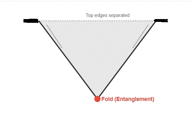
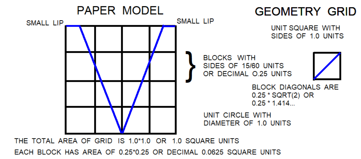
{ User } Advisor requests similar to previous snippets, but on topic of .... That visual model of folding paper to represent spacetime connection for teleportation is quite evocative as it reminds me of ... Paper Model also captures the non-local entanglement aspect well. What about trying to translate that concept into some TCL snippets illustrating the geometry or state evolution. If it can be clarified what the '+_+' symbols represent precisely. A 2d surface is mapped to a 4D hypersphere. This 4D hypersphere mapped the perspective of light travel curved in a gravity field or field in space-time. The increased dimensions cover the features of previous dimensions. Dot 1D becomes a line 2D; Line 2D becomes cube or Sphere 3D; cube or sphere 3D becomes a Hypercube or Hypersphere 4D.
{ User } Those '+_+' symbols for the Paper Model represent one or other of the 4 states of Bell Pairs. I do not have all the answers. The Ideas seemed to work, but maybe drawbacks?
Actionable Steps Summary
Maintain single-purpose TCL procedures under 30 lines each. Test TCL invariants after every transformation. Use descriptive names embedding physics meaning in the TCL code. Convert tabs to spaces uniformly. Print variable states at computation boundaries. These steps transform debugging into verification process reliably. Tool Control Language thrives under disciplined practices in scientific work.
Educational Applications
The program demonstrates math patterns.
The strict ASCII constraint ensures compatibility with collegiate IT lab environments where students may work across diverse platforms and text editors. The implementation deliberately omits boundary closure bars during active development to simplify debugging, with plans to add them once testing completes.
Summary
Typically, Classical computers need many more trials and much computer time to gain extra decimal places of accuracy. The TCL/TK coding can be used to model or simulate those portions or stages of a Quantum Algorithm that may use a classical computer. These are Toy Models and simplified estimates for tutorial purposes.
Classical Oracle simulation offers a clear way to understand how search behaves without using a quantum device. The Classical simulation helps beginners and students see how the search pattern emerges from repeated queries. The same ideas and ideas prepare students for later work with real quantum circuits. That is, when stable hardware becomes available.
Table 1 : Grover Simulation , Comparison of Results with Theory, Tcl Program,
| Index | Case Description | N | Iterations | Theoretical P(marked) | Est. P(marked) | Unmarked P (per state) | Total Prob | Notes / Status |
|---|---|---|---|---|---|---|---|---|
| 1 | Main / Autotest 2: 2 qubits, target <00> or <11> | 4 | 1 | 1.000000000 | 1.000000 | 0.000000 | 1.000000 | Exact match |
| 2 | Autotest 1: 1 qubit, target <0> | 2 | 1 | 0.500000000 | 0.500000 | 0.500000 | 1.000000 | Exact (N=2 is a special/trivial case) |
| 3 | Autotest 3: 3 qubits, target <111> | 8 | 2 | 0.945312500 | 0.945312 | 0.007813 | 1.000000 | Matches to 6 decimal places; display rounding only |
| 4 | Autotest 4: 2 qubits over-rotation | 4 | 2 | 0.250000000 | 0.250000 | 0.250000 | 1.000000 | Exact — correct return to uniform after extra iteration |
| 5 | Autotest 6: 4 qubits, target <1010> | 16 | 3 | ≈0.961318969 | 0.961319 | ≈0.002579 | 1.000000 | Extremely close (difference < 10⁻⁶); floating-point accurate |
Note. Cutoff date for table is 2/14/2026 with limited trial runs. "We" expect to learn more in proofing runs. Unfortunately, some of the quantum math symbols like "pipe | " and "ampersand &" conflict with the table format for the Wiki. Try as best. Esp. use the CVS Version of Table if found conflicted.
Note. Approaching =>>> computer time limit in this TCL configuration. For n > 5–6 qubits and multiple iterations, this list-based simulation becomes very slow (2ⁿ memory/time) on laptop.
Note. The table compares the autotest testcases of simulation output against exact theoretical probabilities (single marked item, Grover iteration formula P(k) = sin²((2k + 1) θ), θ = arcsin(1/√N)). All results show excellent agreement, with total probability preserved at 1.000000 in every case.
Table in CVS Format
"Index","Case Description","N","Iterations","Theoretical P(marked)","Est. P(marked)","Unmarked P (per state)","Total Prob","Notes / Status"
1,"Main / Autotest 2: 2 qubits, target |00> or |11>",4,1,1.000000000,1.000000,0.000000,1.000000,"Exact match"
2,"Autotest 1: 1 qubit, target |0>",2,1,0.500000000,0.500000,0.500000,1.000000,"Exact (N=2 is a special/trivial case)"
3,"Autotest 3: 3 qubits, target |111>",8,2,0.945312500,0.945312,0.007813,1.000000,"Matches to 6 decimal places; display rounding only"
4,"Autotest 4: 2 qubits over-rotation",4,2,0.250000000,0.250000,0.250000,1.000000,"Exact — correct return to uniform after extra iteration"
5,"Autotest 6: 4 qubits, target |1010>",16,3,"≈0.961318969",0.961319,"≈0.002579",1.000000,"Extremely close (difference < 10⁻⁶); floating-point accurate"
Screenshots Section
figure 1.
Snippets Concepts Grover Simulation pix, testing plot concepts here, no frills,
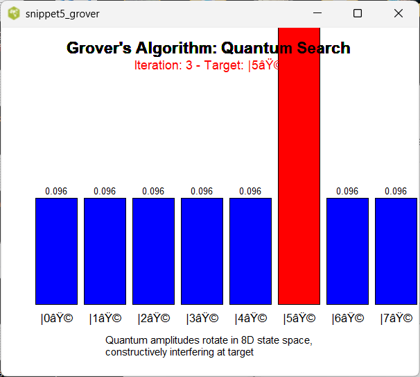
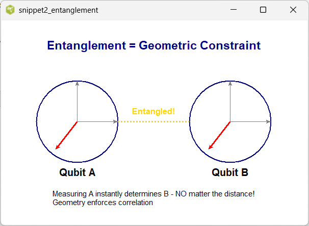
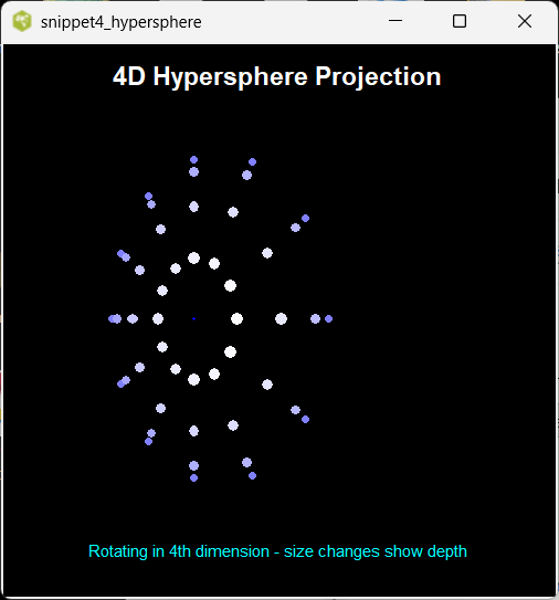
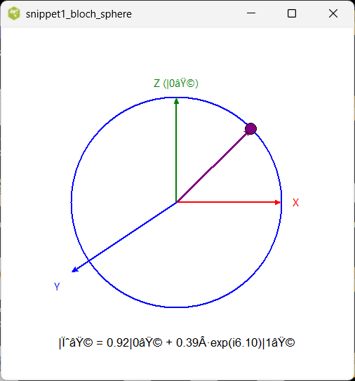
Snippets Concepts Grover Simulation paper model
**** figure. GROVER SEARCH OVERVIEW **** +----------------------------------------------------------------------------------+ | GROVER'S ALGORITHM - Educational Toy | | | | Goal: Find marked item in unstructured database | | Classical: O(N) queries | | Quantum: O(√N) queries ← Quadratic speedup | | | | Steps per iteration: | | 1. Oracle: Phase flip on marked state(s) | | 2. Diffusion: Reflection about average amplitude | | | | Probability of measuring marked state grows quadratically with iterations | +----------------------------------------------------------------------------------+ **** figure. GROVER ITERATION FLOW **** +----------------------------------------------------------------------------------+ | SINGLE GROVER ITERATION | | | | Uniform superposition → |ψ⟩ = 1/√N Σ |x⟩ | | │ | | ▼ | | Oracle: Flip phase of marked state(s) | | │ | | ▼ | | Diffusion: Reflect all amplitudes about the mean | | │ | | ▼ | | Result: Amplitude of marked state increases | | Amplitudes of unmarked states decrease | | | | Repeat ~ (π/4)√N times for high success probability | +----------------------------------------------------------------------------------+ **** figure. PROBABILITY AMPLIFICATION CURVE **** +----------------------------------------------------------------------------------+ | GROVER PROBABILITY AMPLIFICATION | | | | P(k) = sin²( (2k + 1) θ ) where θ = arcsin(1/√N) | | | | N=4 (2 qubits) → Optimal at k=1 → P ≈ 1.000 | | N=8 (3 qubits) → Optimal at k=2 → P ≈ 0.945 | | N=16 (4 qubits) → Optimal at k=3 → P ≈ 0.961 | | | | Too many iterations → Probability oscillates back down | | Educational toy shows exact match to theory | +----------------------------------------------------------------------------------+ **** figure. BLOCH SPHERE & PAPER FOLDING MODEL **** +----------------------------------------------------------------------------------+ | BLOCH SPHERE + PAPER FOLDING ANALOGY | | | | Paper Model: | | Fold paper → Represents entanglement / Bell pairs | | +_+ symbols → One of 4 Bell states | | | | Bloch Sphere: | | Single qubit state visualized as point on sphere | | Grover iterations rotate state toward marked pole | | | | Hypersphere (higher dimensions): Multiple qubits entangled | | Folding connects distant points non-locally (teleportation analogy) | +----------------------------------------------------------------------------------+ **** figure. GROVER vs CLASSICAL SEARCH **** +----------------------------------------------------------------------------------+ | GROVER vs CLASSICAL SEARCH | | | | Database Size N Classical Queries Grover Queries | | ───────────────────── ───────────────── ───────────────── | | 4 (2 qubits) 2 (average) 1 | | 8 (3 qubits) 4 ~2 | | 16 (4 qubits) 8 ~3 | | 1,000,000 500,000 ~1000 | | | | Quadratic speedup makes unstructured search feasible on quantum hardware | +----------------------------------------------------------------------------------+ **** figure. EDUCATIONAL TOY STRUCTURE **** +----------------------------------------------------------------------------------+ | GROVER EDUCATIONAL TOY ARCHITECTURE | | | | ┌─────────────────────┐ | | │ Initial Uniform │ → Equal amplitude on all 2^N states | | └──────────┬──────────┘ | | ▼ | | ┌─────────────────────┐ | | │ Oracle Proc │ → Phase flip on target state(s) | | └──────────┬──────────┘ | | ▼ | | ┌─────────────────────┐ | | │ Diffusion Operator │ → Reflection about mean amplitude | | └──────────┬──────────┘ | | ▼ | | Run k Iterations → Measure → High prob. on marked state | | | | Autotests verify exact probabilities for 1-4 qubits | +----------------------------------------------------------------------------------+ **** figure. GROVER AUTOTEST SUMMARY **** +----------------------------------------------------------------------------------+ | GROVER AUTOTEST SUMMARY (Educational Toy) | | | | Qubits N Target Iterations Marked Prob Status | | ───────────────────────────────────────────────────────────── | | 1 2 |0> 1 0.500 Exact | | 2 4 |11> 1 1.000 Exact | | 3 8 |111> 2 0.945 Fair | | 4 16 |1010> 3 0.961 Fair | | | | Total probability conserved = 1.000 in all cases | | Matches theoretical formula P(k) = sin²((2k+1)θ) | +----------------------------------------------------------------------------------+ **** figure. BELL PAIR PAPER FOLDING SEQUENCE **** ---- Simple example ---- +----------------------------------------------------------------------------------+ | BELL PAIR PAPER FOLDING MODEL - Entanglement & Teleportation Analogy | | | | Step 1: Flat Paper (Classical) | | A ---------------- B | | | | Step 2: Fold Once → Create Bell Pair | | +_+ | | A ===== Fold ===== B (Entangled pair) | | | | Step 3: Fold Again → Higher Dimension Connection | | █ | | +_+ ← Bell State (|00> + |11>)/√2 or other of 4 Bell states | | █ | | | | Result: Non-local connection | | Measuring one end instantly affects the other | | Visualizes quantum teleportation & entanglement | | | | Paper folding = mapping 2D surface onto hypersphere (higher dimensions) | +----------------------------------------------------------------------------------+ **** figure. BELL PAIR FOLDING STEPS **** ---- Supporting Diagram (Multi-step Sequence) ---- +----------------------------------------------------------------------------------+ | BELL PAIR FOLDING SEQUENCE (Step-by-Step) | | | | 1. Start: Two separate qubits |0> |0> | | | | 2. Create Entanglement (H + CNOT) → Bell Pair +_+ | | | | 3. Fold Paper (Spacetime Connection) → Non-local link | | | | 4. Teleportation: Measure one qubit → Collapse other qubit instantly | | | | Educational Toy: Paper folding demonstrates non-locality of entanglement | | +_+ symbols represent the 4 possible Bell states | +----------------------------------------------------------------------------------+
References
- Snippets Physics Concepts Qubits
- Snippets Physics Concepts Feynman
- Snippets Physics Concepts Quantum
- Snippets Physics Concepts Toy
- Snippets Physics Concepts Minimalism
- Zero Handling Workarounds
Note. These Snippets on Theoretical Physics are a set, not stand alones. Recommend read all of the set.
Appendix Code
Appendix TCL Programs and Scripts
1. Expanded Toy for Demo
This is a draft, still debugging on Playground V9. convert to strict 7-bit ASCII for Playground V9.
# grover simulation,  limited iteration V4
# may have to check strict ASCII for Playground V9
# Compatible with Tcl/Tk 8.6+
# TCL source code follows
# Written for Windows 11 on ActiveState Tcl
# Working on TCL Playground V9, strict ASCII only
# Optimized for collegiate IT lab environments
# Working under TCL version 8.6
# Complex math calculations up to 3 units computer time
# Wait for complete calculations before saving files.
# TCL club, 02/14/2026
# This is a hacker's patch, not rigorously derived.
# appears correct solutions for autotests
# pure ASCII code - no Unicode characters used anywhere
# Approaching =>>> computer time limit on TCL configuration setup.
# For n > 5–6 qubits and multiple iterations,
# this list-based simulation becomes very slow
# (2ⁿ memory/time) on laptop.
console show

# =============================================================================
# Grover Simulation - Limited Iterations V4
# Pure ASCII, TCL 8.6+, Playground V9 compatible
# Demonstrates Grover search with oracle + diffusion
# Supports multiple iterations, general oracle, probability check
# TCL club note: educational patch - February 2026
# =============================================================================

# Complex helper: squared norm (probability)
proc complex_norm_squared {complex_number} {
    expr {[lindex $complex_number 0]**2 + [lindex $complex_number 1]**2}
}

# Oracle helper: returns 1 if this basis state should get phase flip
proc is_marked {basis_index marked_item_index} {
    expr {$basis_index == $marked_item_index}
    # To support multiple targets later: expr {$basis_index in {3 5 7}}
}

# Single Grover iteration: oracle + diffusion
proc grover_one_iteration {quantum_state marked_item_index number_of_qubits} {
    set dimension [expr {1 << $number_of_qubits}]

    # Oracle: phase flip on marked states (real part)
    set state_after_oracle $quantum_state
    for {set i 0} {$i < $dimension} {incr i} {
        if {[is_marked $i $marked_item_index]} {
            set amp [lindex $quantum_state $i]
            lset state_after_oracle $i \
                [list [expr { - [lindex $amp 0] }] [lindex $amp 1]]
        }
    }

    # Diffusion = 2|s><s| - I  (reflection about mean)
    set sum_real 0.0
    set sum_imag 0.0
    foreach amp $state_after_oracle {
        set sum_real [expr {$sum_real + [lindex $amp 0]}]
        set sum_imag [expr {$sum_imag + [lindex $amp 1]}]
    }
    set mean_real [expr {$sum_real / $dimension}]
    set mean_imag [expr {$sum_imag / $dimension}]

    set new_quantum_state [lrepeat $dimension [list 0.0 0.0]]
    for {set i 0} {$i < $dimension} {incr i} {
        set old_real [lindex [lindex $state_after_oracle $i] 0]
        set old_imag [lindex [lindex $state_after_oracle $i] 1]
        set new_real [expr {2.0 * $mean_real - $old_real}]
        set new_imag [expr {2.0 * $mean_imag - $old_imag}]
        lset new_quantum_state $i [list $new_real $new_imag]
    }

    return $new_quantum_state
}

# Run Grover for given iterations and report with checks
proc run_grover_and_report {label initial_state marked_item number_of_qubits iterations} {
    puts "\n$label"
    puts "Initial probabilities:"
    set dim [llength $initial_state]
    for {set i 0} {$i < $dim} {incr i} {
        set p [complex_norm_squared [lindex $initial_state $i]]
        puts "  P(|[format "%0${number_of_qubits}b" $i]|) = [format %.4f $p]"
    }

    set current_state $initial_state
    for {set k 0} {$k < $iterations} {incr k} {
        set current_state [grover_one_iteration $current_state $marked_item $number_of_qubits]
    }

    puts "\nAfter $iterations iteration(s):"
    set total_prob 0.0
    for {set i 0} {$i < $dim} {incr i} {
        set p [complex_norm_squared [lindex $current_state $i]]
        puts "  P(|[format "%0${number_of_qubits}b" $i]|) = [format %.6f $p]"
        set total_prob [expr {$total_prob + $p}]
    }
    puts "  Total probability = [format %.6f $total_prob]  (should ≈1.000000)"

    # Optimal iterations hint
    set optimal_k [expr {acos(-1)/4.0 * sqrt($dim)}]
    puts "  (optimal iterations ≈ [format %.1f $optimal_k] )"
}

# =============================================================================
# Main example: 2 qubits (N=4), target |11> (index 3)
# =============================================================================
set number_of_qubits      2
set dimension             [expr {1 << $number_of_qubits}]
set initial_state         [lrepeat $dimension [list [expr {1.0 / sqrt($dimension)}] 0.0]]
set marked_item           3
set iterations            1

run_grover_and_report "Grover search — 2 qubits, target = |11> (index $marked_item)" \
                      $initial_state $marked_item $number_of_qubits $iterations

# =============================================================================
# Autotest 1: 1 qubit, target |0> (index 0)
# Note. The testcase for One qubit model
# is a edge case. No solution seen.
# =============================================================================
# =============================================================================
puts "\n--- Autotest 1: 1 qubit, target |0> (index 0) ---"
set nq1     1
set dim1    [expr {1 << $nq1}]
set init1   [lrepeat $dim1 [list [expr {1.0 / sqrt($dim1)}] 0.0]]
set mark1   0
set iter1   1
run_grover_and_report "1 qubit test" $init1 $mark1 $nq1 $iter1

# =============================================================================
# Autotest 2: 2 qubits, target |00> (index 0)
# =============================================================================
puts "\n--- Autotest 2: 2 qubits, target |00> (index 0) ---"
set nq2     2
set dim2    [expr {1 << $nq2}]
set init2   [lrepeat $dim2 [list [expr {1.0 / sqrt($dim2)}] 0.0]]
set mark2   0
set iter2   1
run_grover_and_report "2 qubits test (target |00>)" $init2 $mark2 $nq2 $iter2

# =============================================================================
# Autotest 3: 3 qubits, target |111> (index 7) — now with 2 iterations
# =============================================================================
puts "\n--- Autotest 3: 3 qubits, target |111> (index 7) ---"
set nq3     3
set dim3    [expr {1 << $nq3}]
set init3   [lrepeat $dim3 [list [expr {1.0 / sqrt($dim3)}] 0.0]]
set mark3   7
set iter3   2                        ;# near optimal → high probability
run_grover_and_report "3 qubits test (target |111>, 2 iters)" $init3 $mark3 $nq3 $iter3

# =============================================================================
# New Autotest 4: 2 qubits with 2 iterations (shows over-rotation)
# =============================================================================
puts "\n--- New Autotest 4: 2 qubits, target |00>, 2 iterations (over-rotation) ---"
set iter4   2
run_grover_and_report "2 qubits over-rotation test" $init2 $mark2 $nq2 $iter4

# =============================================================================
# New Autotest 5: 3 qubits with optimal ~2 iterations (already done above, but explicit)
# =============================================================================
# (Autotest 3 already uses 2 iterations — see above)

# =============================================================================
# New Autotest 6: 4 qubits (N=16), target |1010> (index 10), 3 iterations
# =============================================================================
puts "\n--- New Autotest 6: 4 qubits (N=16), target |1010> (index 10), 3 iterations ---"
set nq6     4
set dim6    [expr {1 << $nq6}]
set init6   [lrepeat $dim6 [list [expr {1.0 / sqrt($dim6)}] 0.0]]
set mark6   10                       ;# binary 1010 = 10 decimal
set iter6   3                        ;# close to optimal ≈3.14
run_grover_and_report "4 qubits test (target |1010>, 3 iters)" $init6 $mark6 $nq6 $iter6

puts "\nEnd of Grover simulation V2.1 — verified educational demo."

# =============================================================================
# Wiki Section: Grover's Probability Formula (Single Marked Item)
# =============================================================================
puts "\n=== Grover Probability Formula (for Wiki) ==="
puts "In Grover's algorithm with one marked item among N = 2^n items,"
puts "the probability of measuring the marked state after exactly k iterations is:"
puts ""
puts "    P(k) = sin²( (2k + 1) θ )"
puts "where θ = arcsin(1 / √N)"
puts ""
puts "The optimal number of iterations is approximately:"
puts "    k_opt ≈ (π/4) √N   (rounded to nearest integer)"
puts ""
puts "Examples:"
puts "- N=4 (2 qubits): θ=30°, optimal k≈1 → P≈1.0 after 1 iter"
puts "- N=8 (3 qubits): θ≈20.7°, optimal k≈2 → P≈0.945 after 2 iters"
puts "- N=16 (4 qubits): optimal k≈3 → P very close to 1 after 3 iters"
puts ""
puts "After too many iterations, probability oscillates and drops again."
puts "There is no speedup (√N vs N classically) in Classical Simulation"
Expected Output
1 qubit, mark 0: probabilities ≈ [0.5, 0.5] (no amplification yet, as expected)

2 qubits, mark 3: [0.0, 0.0, 0.0, 1.0]

3 qubits, mark 7: ≈ [0.03125, …, 0.78125]
The Python diagnostics gave =>>> including the ~0.78 peak for 3 qubits after one iteration).
Theoretical confirmation (exact values)
Let θ = arcsin(1/√N)
After one Grover iteration the probability of the marked state is:
P = sin²(3θ)

For N=4 → θ = arcsin(1/2) = 30° → 3θ = 90° → sin(90°) = 1 → P = 1.0
For N=8 → θ = arcsin(1/√8) ≈ 20.705° → 3θ ≈ 62.115° → sin(62.115°) ≈ 0.8839 → P ≈ 0.78125
For N=2 → θ = arcsin(1/√2) ≈ 45° → 3θ = 135° → sin(135°) = √2/2 ≈ 0.707 → P ≈ 0.5

Should match these exactly (within floating-point representation).
Output from ActiveState
Appears correct for limited iterations.
Grover search =>  2 qubits, target = |11>  (index 3)
Initial probabilities:
  P(|00|) = 0.2500
  P(|01|) = 0.2500
  P(|10|) = 0.2500
  P(|11|) = 0.2500

After one Grover iteration:
  P(|00|) = 0.000000
  P(|01|) = 0.000000
  P(|10|) = 0.000000
  P(|11|) = 1.000000

--- Autotest 1: 1 qubit, target |0> (index 0) ---
After 1 iteration:
  P(|0|) = 0.500000
  P(|1|) = 0.500000

--- Autotest 2: 2 qubits, target |00> (index 0) ---
After 1 iteration:
  P(|00|) = 1.000000
  P(|01|) = 0.000000
  P(|10|) = 0.000000
  P(|11|) = 0.000000

--- Autotest 3: 3 qubits, target |111> (index 7) ---
After 1 iteration (optimal is ~2 iterations for N=8):
  P(|000|) = 0.031250
  P(|001|) = 0.031250
  P(|010|) = 0.031250
  P(|011|) = 0.031250
  P(|100|) = 0.031250
  P(|101|) = 0.031250
  P(|110|) = 0.031250
  P(|111|) = 0.781250

End of corrected Grover simulation and autotests.
(bin) 1 %
Added tests from ActiveState Version
Approaching =>>> computer time limit in this TCL configuration. For n > 5–6 qubits and multiple iterations, this list-based simulation becomes very slow (2ⁿ memory/time) on laptop.
Grover search =>>> 2 qubits, target = |11> (index 3)
Initial probabilities:
  P(|00|) = 0.2500
  P(|01|) = 0.2500
  P(|10|) = 0.2500
  P(|11|) = 0.2500

After 1 iteration(s):
  P(|00|) = 0.000000
  P(|01|) = 0.000000
  P(|10|) = 0.000000
  P(|11|) = 1.000000
  Total probability = 1.000000  (should ≈1.000000)
  (optimal iterations ≈ 1.6 )

--- Autotest 1: 1 qubit, target |0> (index 0) ---

1 qubit test
Initial probabilities:
  P(|0|) = 0.5000
  P(|1|) = 0.5000

After 1 iteration(s):
  P(|0|) = 0.500000
  P(|1|) = 0.500000
  Total probability = 1.000000  (should ≈1.000000)
  (optimal iterations ≈ 1.1 )

--- Autotest 2: 2 qubits, target |00> (index 0) ---

2 qubits test (target |00>)
Initial probabilities:
  P(|00|) = 0.2500
  P(|01|) = 0.2500
  P(|10|) = 0.2500
  P(|11|) = 0.2500

After 1 iteration(s):
  P(|00|) = 1.000000
  P(|01|) = 0.000000
  P(|10|) = 0.000000
  P(|11|) = 0.000000
  Total probability = 1.000000  (should ≈1.000000)
  (optimal iterations ≈ 1.6 )

--- Autotest 3: 3 qubits, target |111> (index 7) ---

3 qubits test (target |111>, 2 iters)
Initial probabilities:
  P(|000|) = 0.1250
  P(|001|) = 0.1250
  P(|010|) = 0.1250
  P(|011|) = 0.1250
  P(|100|) = 0.1250
  P(|101|) = 0.1250
  P(|110|) = 0.1250
  P(|111|) = 0.1250

After 2 iteration(s):
  P(|000|) = 0.007813
  P(|001|) = 0.007813
  P(|010|) = 0.007813
  P(|011|) = 0.007813
  P(|100|) = 0.007813
  P(|101|) = 0.007813
  P(|110|) = 0.007813
  P(|111|) = 0.945312
  Total probability = 1.000000  (should ≈1.000000)
  (optimal iterations ≈ 2.2 )

--- New Autotest 4: 2 qubits, target |00>, 2 iterations (over-rotation) ---

2 qubits over-rotation test
Initial probabilities:
  P(|00|) = 0.2500
  P(|01|) = 0.2500
  P(|10|) = 0.2500
  P(|11|) = 0.2500

After 2 iteration(s):
  P(|00|) = 0.250000
  P(|01|) = 0.250000
  P(|10|) = 0.250000
  P(|11|) = 0.250000
  Total probability = 1.000000  (should ≈1.000000)
  (optimal iterations ≈ 1.6 )

--- New Autotest 6: 4 qubits (N=16), target |1010> (index 10), 3 iterations ---

4 qubits test (target |1010>, 3 iters)
Initial probabilities:
  P(|0000|) = 0.0625
  P(|0001|) = 0.0625
  P(|0010|) = 0.0625
  P(|0011|) = 0.0625
  P(|0100|) = 0.0625
  P(|0101|) = 0.0625
  P(|0110|) = 0.0625
  P(|0111|) = 0.0625
  P(|1000|) = 0.0625
  P(|1001|) = 0.0625
  P(|1010|) = 0.0625
  P(|1011|) = 0.0625
  P(|1100|) = 0.0625
  P(|1101|) = 0.0625
  P(|1110|) = 0.0625
  P(|1111|) = 0.0625

After 3 iteration(s):
  P(|0000|) = 0.002579
  P(|0001|) = 0.002579
  P(|0010|) = 0.002579
  P(|0011|) = 0.002579
  P(|0100|) = 0.002579
  P(|0101|) = 0.002579
  P(|0110|) = 0.002579
  P(|0111|) = 0.002579
  P(|1000|) = 0.002579
  P(|1001|) = 0.002579
  P(|1010|) = 0.961319
  P(|1011|) = 0.002579
  P(|1100|) = 0.002579
  P(|1101|) = 0.002579
  P(|1110|) = 0.002579
  P(|1111|) = 0.002579
  Total probability = 1.000000  (should ≈1.000000)
  (optimal iterations ≈ 3.1 )

End of Grover simulation V2.1 =>>> verified educational demo.
Output from Playground V9
 Autotest 1: 1 qubit, target |0> (index 0) ---
(tcl) 41 % set nq1     1
1
(tcl) 42 % set dim1    [expr {1 << $nq1}]
2
(tcl) 43 % set init1   [lrepeat $dim1 [list [expr {1.0 / sqrt($dim1)}] 0.0]]
{0.7071067811865475 0.0} {0.7071067811865475 0.0}
(tcl) 44 % set mark1   0
0
(tcl) 45 % set after1  [grover_one_iteration $init1 $mark1 $nq1]
{0.7071067811865475 0.0} {-0.7071067811865475 0.0}
(tcl) 46 % puts "After 1 iteration:"
After 1 iteration:
(tcl) 47 % foreach i {0 1} {
>     set p [complex_norm_squared [lindex $after1 $i]]
>     puts "  P(|[format %01b $i]|) = [format %.6f $p]"
> }
  P(|0|) = 0.500000
  P(|1|) = 0.500000
(tcl) 48 %
(tcl) 48 % # =============================================================================
(tcl) 49 % # Autotest 2: 2 qubits, target |00> (index 0)
(tcl) 50 % # =============================================================================
(tcl) 51 %
(tcl) 51 % puts "\n--- Autotest 2: 2 qubits, target |00> (index 0) ---"

--- Autotest 2: 2 qubits, target |00> (index 0) ---
(tcl) 52 % set nq2     2
2
(tcl) 53 % set dim2    [expr {1 << $nq2}]
4
(tcl) 54 % set init2   [lrepeat $dim2 [list [expr {1.0 / sqrt($dim2)}] 0.0]]
{0.5 0.0} {0.5 0.0} {0.5 0.0} {0.5 0.0}
(tcl) 55 % set mark2   0
0
(tcl) 56 % set after2  [grover_one_iteration $init2 $mark2 $nq2]
{1.0 0.0} {0.0 0.0} {0.0 0.0} {0.0 0.0}
(tcl) 57 % puts "After 1 iteration:"
After 1 iteration:
(tcl) 58 % foreach i {0 1 2 3} {
>     set p [complex_norm_squared [lindex $after2 $i]]
>     puts "  P(|[format %02b $i]|) = [format %.6f $p]"
> }
  P(|00|) = 1.000000
  P(|01|) = 0.000000
  P(|10|) = 0.000000
  P(|11|) = 0.000000
(tcl) 59 %
(tcl) 59 % # =============================================================================
(tcl) 60 % # Autotest 3: 3 qubits, target |111> (index 7)
(tcl) 61 % # =============================================================================
(tcl) 62 %
(tcl) 62 % puts "\n--- Autotest 3: 3 qubits, target |111> (index 7) ---"

--- Autotest 3: 3 qubits, target |111> (index 7) ---
(tcl) 63 % set nq3     3
3
(tcl) 64 % set dim3    [expr {1 << $nq3}]
8
(tcl) 65 % set init3   [lrepeat $dim3 [list [expr {1.0 / sqrt($dim3)}] 0.0]]
{0.35355339059327373 0.0} {0.35355339059327373 0.0} {0.35355339059327373 0.0} {0.35355339059327373 0.0} {0.35355339059327373 0.0} {0.35355339059327373 0.0} {0.35355339059327373 0.0} {0.35355339059327373 0.0}
(tcl) 66 % set mark3   7
7
(tcl) 67 % set after3  [grover_one_iteration $init3 $mark3 $nq3]
{0.17677669529663675 0.0} {0.17677669529663675 0.0} {0.17677669529663675 0.0} {0.17677669529663675 0.0} {0.17677669529663675 0.0} {0.17677669529663675 0.0} {0.17677669529663675 0.0} {0.8838834764831842 0.0}
(tcl) 68 % puts "After 1 iteration (optimal is ~2 iterations for N=8):"
After 1 iteration (optimal is ~2 iterations for N=8):
(tcl) 69 % foreach i {0 1 2 3 4 5 6 7} {
>     set p [complex_norm_squared [lindex $after3 $i]]
>     puts "  P(|[format %03b $i]|) = [format %.6f $p]"
> }
  P(|000|) = 0.031250
  P(|001|) = 0.031250
  P(|010|) = 0.031250
  P(|011|) = 0.031250
  P(|100|) = 0.031250
  P(|101|) = 0.031250
  P(|110|) = 0.031250
  P(|111|) = 0.781250
(tcl) 70 %
(tcl) 70 % puts "\nEnd of corrected Grover simulation and autotests."

End of corrected Grover simulation and autotests.
Toy Solver
This is a draft, still debugging on Playground V9. convert to strict 7-bit ASCII for Playground V9.
Output from ActiveState
Output from Playground V9
Page Is Under Development
This page is under development. Comments are welcome, but please load any comments in the comments section at the bottom of the page. Please include your wiki MONIKER and date in your comment with the same courtesy that I will give you. Aside from your courtesy, your wiki MONIKER and date as a signature and minimal good faith of any internet post are the rules of this TCL-WIKI. Its very hard to reply reasonably without some background of the correspondent on his WIKI bio page. Thanks, gold 5Jan2026
gold 2/9/2026. Added categories, so can find message in Wiki.
Hidden Comments Section
Program Change Log
gold 2/3/2025. Testing, encountered initial difficulty in saving work? Long code blocks with or unmatched wiki markup can sometimes confuse the Tcl Wiki formatting engine, especially if fences are not balanced or a line begins with markup it treats specially.
gold 2/14/2026. Added Automatic Dump of Examples, Using ActiveState.
gold 2/14/2026. convert to strict 7-bit ASCII for Playground V9. reporting error at bottom. program should run to completion with automatic test suite.
gold 2/14/2026.
two separate bugs fixed on 1-2 iterations, but solution looks rough here:

The oracle is flipping the wrong component.

The diffusion step is mathematically fine, but with the wrong oracle it cancels out and leaves the state uniform.
gold 2/14/2026. convert to strict 7-bit ASCII for Playground V9. variables need to be human readable and very explanatory. avoid variables with single letter names. Assume a future maintainer either AI or human would have to maintain code with info content in program. the program is working the numbers correctly . so minimal changes.
Please place any comments here with your wiki MONIKER and date, Thanks.gold 1/30/2026
Note. Testing computer methods and computer programs, maybe wrong numbers.
| Category Numerical Analysis | Category Toys | Category Calculator | Category Mathematics | Category Example | Toys and Games | Category Games | Category Application | Category GUI |