Sampled Signal Reconstruction in Tcl driven Maxima
started by Theo Verelst
Maxima is a tcl-containing math program with Tk interface. In this example tcl is used to fabricate formulas for maxima's interpreter, for a part of one of the most important issues in signal processing and computerized real-world data interaction: the reconstruction of a sampled signal.
continuous real-life / physical signal ---> sampled, time discrete signal ---> reconstructed signal
Important for people using for instance snack, the tcl/tk sound sample and process library, and especially if that use includes measurement-like analyisis, which is quite reasonably possible with tcl, and essential for anybody in signal processing type of field, or let's say where measurements are taken and actuators driven by tcl (and tk).
The whole subject is basis years advanced EE stuff, but the essence is that when a signal (like a sound source for snack) is sampled, or when peole play around with 'signal vectors' and possibly matrix-based or other signal operations in tcl, or even when functions are plotted with Tk (refs?) based on a limited set of evaluated points, once the samples in a list or array are supposed to be interprerted or transformed back as continuous signal , the usual DA converter or step (0th order) approximation does not do a very good job at doing justice to the theory behind sampling.
In this example I used maxima to construct a signal of artificial samples of a frequency-spectrum-limited square wave approximation, as to fulfill Shannon sampling theorem conditions for the example (no frequencies lower than 1/2 sampling frequency).
frequency limited square wave approximation --> small number of equidistant samples --> reconstructed continuous signal
For reconstructing the continuous signal from samples, the sinc function is important:
 (C4) sinc(x,i):=sin((x-i)*%pi)/((x-i)*%pi);
                                                 SIN((x - i) %PI)
 (D4)                              sinc(x, i) := ----------------
                                                   (x - i) %PI
(C$ is the prompt where I typed after. maxima presents a formula with character-typesetting-based formatting as answer in a Tk text window). I typed from the top of my head; I'm not sure normalization for instance is perfect at all.
The artificial signal of which I make samples is:
 (C16) sq7(t):=sin(2*%pi*t)+(1/3)*sin(3*2*%pi*t)+(1/5)*sin(5*2*%pi*t)+(1/7)*sin(7*2*%pi*t);
                                   1                  1                  1
 (D16)    sq7(t) := SIN(2 %PI t) + - SIN(3 2 %PI t) + - SIN(5 2 %PI t) + - SIN(7 2 %PI t)
                                   3                  5                  7
To make the signal reconstruction formula in a way that I happened to find handy to quickly get to a result, I used 'Show tcl console' from the Options menu, and used the following maxima code generator line in Tcl:
   for {set i 0} {$i<29} {incr i} {
      puts -nonewline "sinc(x,$i)*sq7($i/28)+ "
   }
Which gives all the terms for 28 samples reconstructing a signal made by adding three sine components of a square wave approximation with cycle length 28, sampled at equidistant times 0,1,2...28, where each sample is weighing a sinc function for continuous signal reconstruction.
To define the function in maxima that represents the signal, I used the result of this tcl script to define the res1 function of x, in my case by pasting the outcome of puts (.maxima.text insert current ... would work, too):
 (C54) res1(x):=sinc(x,0)*sq7(0/28)+ sinc(x,1)*sq7(1/28)+ sinc(x,2)*sq7(2/28)+ sinc(x,3)*sq7(3/28)+
 sinc(x,4)*sq7(4/28)+ sinc(x,5)*sq7(5/28)+ sinc(x,6)*sq7(6/28)+ sinc(x,7)*sq7(7/28)+
 sinc(x,8)*sq7(8/28)+ sinc(x,9)*sq7(9/28)+ sinc(x,10)*sq7(10/28)+ sinc(x,11)*sq7(11/28)+
 sinc(x,12)*sq7(12/28)+ sinc(x,13)*sq7(13/28)+ sinc(x,14)*sq7(14/28)+ sinc(x,15)*sq7(15/28)+
 sinc(x,16)*sq7(16/28)+ sinc(x,17)*sq7(17/28)+ sinc(x,18)*sq7(18/28)+ sinc(x,19)*sq7(19/28)+
 sinc(x,20)*sq7(20/28)+ sinc(x,21)*sq7(21/28)+ sinc(x,22)*sq7(22/28)+ sinc(x,23)*sq7(23/28)+
 sinc(x,24)*sq7(24/28)+ sinc(x,25)*sq7(25/28)+ sinc(x,26)*sq7(26/28)+ sinc(x,27)*sq7(27/28);
                                  0                    1                    2                    3
 (D54) res1(x) := sinc(x, 0) sq7(--) + sinc(x, 1) sq7(--) + sinc(x, 2) sq7(--) + sinc(x, 3) sq7(--)
                                 28                   28                   28                   28

                   4                    5                    6                    7
 + sinc(x, 4) sq7(--) + sinc(x, 5) sq7(--) + sinc(x, 6) sq7(--) + sinc(x, 7) sq7(--)
                  28                   28                   28                   28

                   8                    9                    10                    11
 + sinc(x, 8) sq7(--) + sinc(x, 9) sq7(--) + sinc(x, 10) sq7(--) + sinc(x, 11) sq7(--)
                  28                   28                    28                    28

                   12                    13                    14                    15
 + sinc(x, 12) sq7(--) + sinc(x, 13) sq7(--) + sinc(x, 14) sq7(--) + sinc(x, 15) sq7(--)
                   28                    28                    28                    28

                   16                    17                    18                    19
 + sinc(x, 16) sq7(--) + sinc(x, 17) sq7(--) + sinc(x, 18) sq7(--) + sinc(x, 19) sq7(--)
                   28                    28                    28                    28

                   20                    21                    22                    23
 + sinc(x, 20) sq7(--) + sinc(x, 21) sq7(--) + sinc(x, 22) sq7(--) + sinc(x, 23) sq7(--)
                   28                    28                    28                    28

                   24                    25                    26                    27
 + sinc(x, 24) sq7(--) + sinc(x, 25) sq7(--) + sinc(x, 26) sq7(--) + sinc(x, 27) sq7(--)
                   28                    28                    28                    28
 (C55) plot2d(res1(x),[x,-10.01,31.99],[y,-1.5,1.5],[nticks,800]);
This example makes the error that the influence of each sample on the resulting (reconstructed) signal, extends pretty far, because the 1/x term doesn't vanish quickly, while the definition of the reconstruction function requires that each term from - through + infinity is taken into account. The resulting graph (I've prevented the sin(x)/x 0 limit case by slightly offsetting the graphing to prevent dividion by 0):
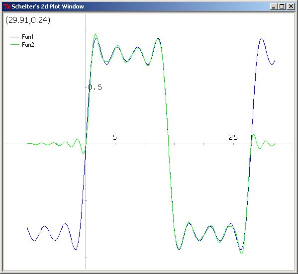
The plot line in maxima (note again you can use tcl and tk to input commmands to the maxima interpreter):
plot2d([sq7(x/28),res1(x)],[x,-10,32],[y,-1.5,1.5],[nticks,800]);
By taking 28 samples before and after the wave we viewed into account as well, results visually start to become more accurate, though beware that when you play back samples over snack, a good quality audio setup will make errors in the sub 0.01% range audible, which snack can in principle handle by using 16-bit samples, but the above shows that the DA converter would have to weight possibly up to 10,000 samples before and after each sample to prevent sync-function-error-induced recontruction errors ([expr sin($x)/$x] is down to 0.0001 for x > 10000 ...) .
The tcl formula generator now was:
for {set i -28} {$i<2*28} {incr i} {puts -nonewline "sinc(x,$i)*sq7($i/28)+ "}
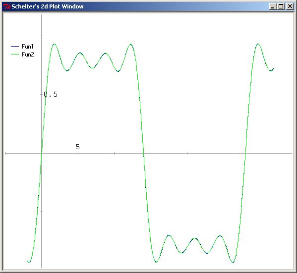
Clearly better.
Notice that by the use of tcl a formula generator, combined with the maxima symbolic computation engine, a powerfull result has been made, which in principle could be, apart from plotting, used for subsequent mathematical analysis.
An important concept for computer represented signals or changing variables which are in fact continuous, is how a signal develops with time, such as I examplified with snack in Sound envelope generator . The exceptional relevance of this is that as soon as a signal is made time limited somehow, as even smoothly is done with that examples, the official fourier transform of the signal (the frequencies supposedly present in the signal) becomes infinite, and that has as immedeate and grave consequence that it isn't officially possible anymore to sample that signal, and reconstruct it from the samples without error! Then there is always a aliasing error ! Considering digital computers exclusively can work with sampled, time and even amplitude discrete, signals, and that many computer models and uses involve signals which in real life mostly can be thought to be time continuous, ranging from cell membrane voltage representations over audio and video (2D sampled!) to database representations of real-life values such as in expert systems, this is a very serious and noteworthy limitation and source of errors, often seriously overlooked. A lot of computer humbug can be prevented by disallowing computer based views which do not take this important and fundamental theory into account.