Sine wave roundings illustrated with BWise

started by Theo Verelst

When dealing with the solution of (2d order) differential equations, electrical circuits, drawing circles, making musical waves or fourier analysis, sine waves or sine values as function of lets say x are essential.

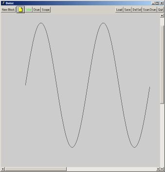
Lets first draw a sine wave with a reasonable graphical accuracy, make sure you have a (preferably scrollable) Tk canvas to work on, and that the tcl variable mc contains the path to that canvas.

This routine, called with the number of x-steps draws 2 periods of a sine wave, with 1:1 x:y scale ratio, and rouding of y coordinates by truncation:

proc drawsine { {n 256} } {
    global mc
    set pi 3.1415926535
    $mc del gr
    for {set i 1} {$i < 2*$n} {incr i} {
        $mc create line [expr 100+$i-1] \
            [expr 100+$n-$n*sin(2*$pi*($i-1)/$n)] \
            [expr 100+$i] \
            [expr 100+$n-$n*sin(2*$pi*($i)/$n)] \
                -tag gr
    }
}

drawsine 256

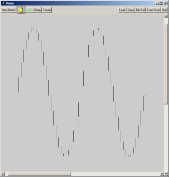
Now when we make the y coordinate quantized per 10 of the above pixel widths

proc drawsine_yq { {n 256} } {
    global mc
    set pi 3.1415926535
    $mc del gr
    for {set i 1} {$i < 2*$n} {incr i} {
        $mc create line [expr 100+$i-1] \
            [expr 100+$n-$n*sin(2*$pi*10*int(($i-1)/10)/$n)] \
            [expr 100+$i] \
            [expr 100+$n-$n*sin(2*$pi*10*int(($i)/10)/$n)] \
                -tag gr
    }
}

proc drawsine_yq { {n 256} } {
    global mc
    set pi 3.1415926535
    $mc del gr
    for {set i 1} {$i < 2*$n} {incr i} {
        $mc create line [expr 100+$i-1] \
            [expr 100+$n-$n*sin(2*$pi*10*int(($i-1)/10)/$n)] \
            [expr 100+$i] \
            [expr 100+$n-$n*sin(2*$pi*10*int(($i-1)/10)/$n)] \
                -tag gr
    }
}

drawsine_yq 256

the graph looks like above, depending on whether the vertical connection lines are drawn or not.

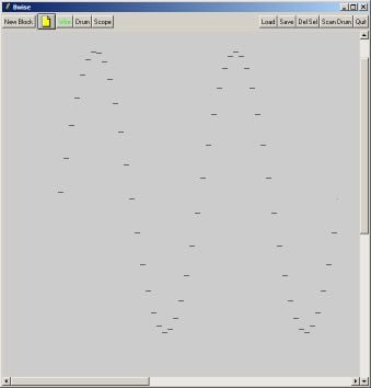
Alternatively, we can clearly (because even with double accuracy floating point numbers, computer accuracy isn't infinite) quantize the x coordinates, and then interpolate somehow:

proc drawsine_xq { {n 256} } {
    global mc
    set pi 3.1415926535
    $mc del gr
    for {set i 1} {$i < 2*$n} {incr i} {
        $mc create line [expr 100+10*int(($i-1)/10)] \
            [expr 100+$n-$n*sin(2*$pi*($i-1)/$n)] \
            [expr 100+10*int(($i-1)/10)] \
            [expr 100+$n-$n*sin(2*$pi*$i/$n)] \
                -tag gr
    }
}

Note that in the case of Y quantisation there are equal distances of 10 between all y values in the graph, and for X quantisation, the X coordinates are rounded to a fixed grid of 10 wide spacing (the images have been shrunk by a factor of 2).

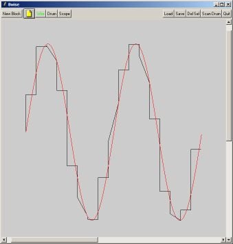
Now if we take a non simple related x and y quantisation and an unclear (though well defined) interpolation strategy, in this case straight line through the sampled points, and make a fairly course quantisation (allow only a few values on the x and y axis where everythingis rounded to), results become maybe artistic, but not very scientifically usable:

proc drawsine_xyq { {n {256}} } {
   global mc
   set pi 3.1415926535
   $mc del gr
   set qx 30
   set qy 18
   for {set i 1} {$i < 2*$n} {incr i} {
      $mc create line [expr 100+$qx*int(($i-1)/$qx)] \
      [expr 100+$n-$n*sin(2*$pi*$qy*int(($i-1)/$qy)/$n)] \
      [expr 100+$qx*int(($i)/$qx)] \
      [expr 100+$n-$n*sin(2*$pi*$qy*int(($i)/$qy)/$n)] \
      -tag gr
   }
} 

Remember, these values aren't rounded, and no attempt is made to make the quantized patterns come as close as possible to the sine wave by any measure such as max or average distance or integral of absolute difference, or of course least square sense or so.

Things get even more hard to follow when sampling and signal reconstruction are also in the signal path.