Snippets Concepts Hypersphere Simulation
- Index for Snippets Concepts Hypersphere Simulation
- Limitations on Tool
- Extra Significant Figures, If Any in Debugging
- Introduction
- Body
- Key Steps
- Draft on Protocol
- Modeled
- PRACTICAL VISUALIZATION AND TIPS
- Rationale and Set of Directions
- Actionable Steps Summary
- Tangerine as Analog model for Hyper-Ellipsoid
- Pseudocode for Orange Tangerine Model
- Analog model for Lossless Arrow Hitting the Celestial Sphere
- Seeking Solutions with Oversimplifications, Dead Ends, and False Starts
- Concepts on Animated GIF89a
- Tweaks needed on Gif?
- Educational Applications
- Table 1 : Comparison of Snippet Utility with Theoretical Physics., Tcl Snippets,
- Table in CVS Format
- Figure. Simulation pix
- Figure. Simulation entanglement
- Figure. Simulation Bloch Sphere
- Figure. Simulation stereo
- Figure. Simulation paper model
- Figure. Model Grid
- Figure. Orange Tangerine Model
- Figure. Analog of Lossless Arrow Hitting Celestial Sphere
- Figure. Mockup on Lossless Arrows Traversing Stellar Neighborhood, Hitting Celestial Sphere
- Figure. Rotating Hypersphere
- Figure. Hypersphere Simulation on Playground V9
- Simulation now HyperEllipsoid
- Figure. Hyper-Ellipsoid with Grid on Reflecting Floor
- Figure. Composite X_ray all_sky image
- Figure. Composite Reflection,
- References
- Appendix Code
- 1. Expanded Toy for Demo
- Output from ActiveState
- Added tests from ActiveState Version
- Toy Solver
- Output from ActiveState
- Output from Playground V9
- Output from ActiveState
- Table on Comparison for Hyper-Ellipsoid Simulation, Python style Pseudocode vs Tcl style Pseudocode equivalent
- Pseudocode Comparison
- Table‑driven pseudocode with comments
- Example inline pseudocode block
- Pseudocode for Gravity Wave Simulation
- Page Is Under Development
- Hidden Comments Section
- Program Change Log
Index for Snippets Concepts Hypersphere Simulation
Preface
gold 2/14/2026. Here are some simple snippets for numerical methods. The goal is to use Tcl's minimalism as a learning tool. Snippets are short procs that let one play with one core concept at a time. All snippets are Playground V9 safe. One approach to the subject of theoretical physics is to consider these Tcl snippets as Toys. Some snippets here are listed as Toys. These Tcl procs are tiny entry points into physics. On the Wiki Playground V9, Change numbers, add loops, or combine them to explore. Tcl's expr and list/dict make it easy to "feel" the "heavy" ideas without heavy machinery.
Limitations on Tool
The TCL Snippets illustrate ideal mathematical behavior only and do not perform full simulation, actual measurements, or state vector evolution. The tool only visualizes ideal math structure, whereas no state vector simulation, probabilities, or actual measurement outcomes are derived. This tool for visualization does not simulate actual measurement outcomes or state vector evolution during operations. These are idealized protocols for tutorial purposes. Primarily, TCL /TK uses its strong points here for book keeping and displays. The example tool is not a full emulator. Meaning, limited scope for tutorial purposes.
Extra Significant Figures, If Any in Debugging
In debugging the calculations, some of the printout values reflect roughly 17-digit precision output from a typical double-precision computation. It's not "true exact" beyond 5 significant figures. Extra significant figures are used to check the calculations from other computer set-ups, not necessarily to infer accuracy of data measurements here. Typically, the slight differences in decimal places on far right of decimal point are normal floating-point behavior in Tcl's expr.
Introduction
The page presents Tcl code snippets. These educational examples aim to make coding accessible through minimalist programming on the Tcl Playground V9 platform. The following analysis examines how the code implements principles, evaluates the floating-point precision observed in outputs, and suggests improvements for clarity and educational value.
Body
Key Steps
Draft on Protocol
gold This is a draft. 2/14/2026
Modeled
{ User } Advisor requests similar to previous snippets, but on topic of .... That visual model of folding paper to represent spacetime connection for teleportation is quite evocative as it reminds me of ... Paper Model also captures the non-local entanglement aspect well. What about trying to translate that concept into some TCL snippets illustrating the geometry or state evolution. If it can be clarified what the '+_+' symbols represent precisely. A 2d surface is mapped to a 4D hypersphere. This 4D hypersphere mapped the perspective of light travel curved in a gravity field or field in space-time. The increased dimensions cover the features of previous dimensions. Dot 1D becomes a line 2D; Line 2D becomes cube or Sphere 3D; cube or sphere 3D becomes a Hypercube or Hypersphere 4D.
{ User } Those '+_+' symbols for the Paper Model represent one or other of the 4 states of Bell Pairs. Advisor has requested Hyper-Ellipsoid model for Space-Time. However, its easier to program the 'mental gymnastics and meaningful pseudocode', if the cards for Wild-Card and Jokers??? are presented up front on the table. I do not have all the answers. The Ideas seemed to work, but maybe drawbacks?
PRACTICAL VISUALIZATION AND TIPS
Rationale and Set of Directions
Gist. What Prof. Sabrina Pasterski is Doing ( Gravity Mapping on Hypersphere?) Pasterski's work -> boundary ... Gravitational information, including memory effects from gravitational waves, soft graviton imprints, resides on this boundary surface. 4D mapping simplifies ER=EPR conjecture.
gold 2/16/2026. editor assistance from 2nd, 2/15/2026
Prof. Sabrina Pasterski is advancing celestial holography, a framework that applies the holographic principle to flat spacetimes with vanishing cosmological constant. This approach seeks to unify gravity described by general relativity with quantum mechanics. The primary purpose of this executive summary is to explain Pasterski's core contributions in accessible terms. The summary highlights the mapping of gravitational information from four-dimensional spacetime to a two-dimensional celestial sphere. The discussion also connects this work to broader implications for quantum gravity.
Celestial holography proposes a duality between the gravitational scattering matrix, known as the S-matrix, in asymptotically flat spacetimes and correlators in a two-dimensional conformal field theory (CFT) living on the celestial sphere. Pasterski and collaborators motivate this duality through asymptotic symmetries, such as BMS (Bondi-Metzner-Sachs) symmetries, which extend Poincaré invariance at infinity. These symmetries manifest in soft theorems for low-energy gravitons. Soft theorems reveal infinite-dimensional enhancements that organize into currents on the celestial sphere. This organization transforms scattering amplitudes into objects that behave like conformal correlators.
The celestial sphere arises from conformal compactification of Minkowski space. This process maps the infinite boundary of spacetime—where light rays reach null infinity—to a finite three-sphere, often simplified to its spatial two-sphere cross-section, the celestial sphere. Researchers sometimes describe this compactified structure in terms of a hypersphere to handle the full asymptotic geometry compactly.
Prof. Pasterski's work emphasizes this boundary encoding. Gravitational information, including memory effects from gravitational waves and soft graviton imprints, resides on this boundary surface. The mapping simplifies complex four-dimensional gravity problems to more tractable two-dimensional quantum field theory calculations. This framework bridges quantum entanglement and spacetime geometry. The ER=EPR conjecture suggests that entangled particles connect via microscopic wormholes. In celestial holography, quantum correlations on the boundary may generate bulk spacetime curvature.
Pasterski explores how conformally soft theorems and operator product expansions encode collinear limits and other structures in amplitudes. Recent developments include bottom-up constructions from symmetries and top-down approaches inspired by string theory or twisted holography. These efforts aim to build a complete holographic dictionary for flat space.
Pasterski's research offers practical gains for quantum gravity. The approach enables computable predictions for gravitational wave observables and black hole information problems. It also inspires applications in quantum information and computing. By treating gravity holographically on the "night sky," celestial holography provides a novel path toward reconciling general relativity with quantum theory in realistic cosmologies. Ongoing work at initiatives like the Celestial Holography Initiative at Perimeter Institute continues to refine this dictionary and explore experimental connections.
Actionable Steps Summary
Maintain single-purpose TCL procedures under 30 lines each. Test TCL invariants after every transformation. Use descriptive names embedding physics meaning in the TCL code. Convert tabs to spaces uniformly. Print variable states at computation boundaries. These steps transform debugging into verification process reliably. Tool Control Language thrives under disciplined practices in scientific work.
Tangerine as Analog model for Hyper-Ellipsoid
I use analogs or simulation models in a new task for TCL programming. Real shape is Hyper-Ellipsoid in 4D. The tangerine figure is distorted by approaching the S-T Anomaly. The internal information field or sweet pulp of the tangerine is implied by the bitterness of the tangerine peel. The bitterness or implied information is contained in pores along the outside of the peel. The Hyper-Ellipsoid in 4D is converted into a ellipsoid in 3d or football shape. Then the sections of the tangerine peel are laid out on a 2D surface. Sections of the peel are laid out flat on the 2D surface, whether the peels are laid out horizontally, side to side, or longitudinally, end to end. The pores of the rind or original information content and possibly distorted pores, are then measured or tallied by a counting or an accumulation function, tabulating pores over surface area. The expanses of information in the S-T field is given by features of 2D shape. The Advisor has yet to characterize the S-T anomaly, but I believe that throwing the tangerine against a wall would give sufficient distortion to Hyper-Ellipsoid for now.
Gravity in the tangerine core has information and "memory" transforms to flattening on the 2D surface. This is the observer problem. Add to the gif, a 2d canted floor below the hyper-ellipsoid 4d to show the "refection" of the hyper-ellipsoid on a 2-D surface. Some explanatory material is loaded on new wiki page. "Snippets Concepts Hypersphere Simulation", but as you know, I work primarily in Tcl.
Pseudocode for Orange Tangerine Model
Lengthy Pseudocode, stacked below Auxiliary Code at bottom.
Credit due. The original framework was developed by Sabrina Pasterski. Prof. Pasterski is a theoretical physicist and pioneer of celestial holography at the Perimeter Institute. Provides the mathematical backbone for this tangerine analogy. Pasterski's work encodes all physical events in asymptotically flat spacetime onto a two-dimensional (2D) boundary called *null infinity*. This boundary behaves like a kind of universal recording surface — a cosmic tangerine peel, if you will — upon which the interior dynamics of four-dimensional (4D) spacetime leave permanent holographic imprints.
To simulate the tangerine analog computationally, one can parameterize the 4D hyper-ellipsoid surface and project it down dimension by dimension. A minimal simulation started from pseudocode (adaptable to Python, TCL, or Julia) might proceed.
A gravitational wave passing through the system perturbs the semi-axes a, b, c, d as a function of time. This can be modeled as a small oscillatory perturbation.
Analog model for Lossless Arrow Hitting the Celestial Sphere
Wow! The questions that I am asked—and the many answers that I don't know. A fellow engineer on the job asked me if my TCL programs can measure gravity. Following the Newton legend and the position measurements with a long string, I can measure the position of the resting apple on the branch and even the resting apple on the ground, relative to the base of the tree. With my long string, I can measure distances relative to the base of the tree and even the trajectory of the apple falling from the tree branch. Given a little depth and more polish to the TCL programs, I can estimate the inertial coordinates of the tree and the trajectory of the apple, in terms of the moving inertial coordinates at the center of Earth’s mass. But my TCL program cannot measure gravity directly or tell me what gravity is. You can see why I am dissatisfied with the analogy of Newton’s apple.
However, let's look at the lossless arrow hitting a target like the Moon, which is positioned on the celestial sphere. Unlike real arrows, the lossless arrow continues on through the Moon to impact the celestial sphere. Effectively, the lossless arrow establishes a vector and impact point ending at infinity on the celestial sphere. Further, the impact or kinetic energy of the lossless arrow can be measured or estimated at the final coordinates on the celestial sphere. So now, we have a resting point on the celestial sphere with an estimated magnitude. However, since the lossless arrow is at rest on the celestial coordinates, the Newtonian rules imply that gravity is not measurable on a resting body.
Note. The proposed snippet fires three arrows from the origin, computes three impact points, and draws three red dots on celestial sphere coordinates. Suggesting that polished up extension on proposed arrow model would have to solve the Einstein equations. A 100x100 pixel grid processes quickly in Tcl. Larger grids or many time steps could slow older laptops.
Seeking Solutions with Oversimplifications, Dead Ends, and False Starts
This gravity problem is effectively a boundary value problem. That is, the solution and the unknown parameters are constrained by the initial conditions and final conditions. It is somewhat like the cannonball problems in high school, where initial velocity, momentum vectors, flight time, and final distance were given, then one had to solve for the cannonball’s flight between the initial conditions and final conditions.
Here is another approach to avoid a flaw in our thinking: sometimes we treat a problem too simply. For example, when solving for the motion of a pendulum bob, we might start with the original and conventional formula. But it turns out that the original formula is oversimplified. A closer, more accurate formula involves a series expansion, solved using series notation.
Simple models for the pendulum bob work well in everyday situations, but they rely on strong simplifications: constant gravity, no air resistance, flat non-rotating Earth, speeds far below light speed, and mass canceling out. In extreme regimes these assumptions break down. Another classic case is the simple pendulum. The small-angle approximation gives the period formula:
# Taciturn simplified formula from math textbooks
T ≈ 2 * pi * sqrt(L / g)
This comes from replacing sin(theta) ≈ theta (in radians) for small swings. The equation of motion becomes linear, like a harmonic oscillator. For larger angles the exact period requires an elliptic integral, which has no simple closed form. A useful series expansion (accurate for moderate angles) is:
# Switching to human readable variables in Tcl
# Basic factor
set basic_formula [expr {2 * acos(-1.0) * sqrt($length / $gravity)}]

# Series correction (first two terms are usually enough)
set correction_factor_from_theta_series [expr {1 + (1.0/16) * pow($max_angle_rad, 2) \
                          + (11.0/3072) * pow($max_angle_rad, 4)}]

set accurate_period [expr {$basic_formula * $correction_factor_from_theta_series}]
where theta0 is the maximum swing angle in radians. The basic formula is convenient, but becomes a dead end when precision is needed for clocks, seismology, and large-amplitude experiments.
Gist. Another example is the cannonball problem from high school, where we treated time, mass, and gravity as constants. But maybe there is an alternate solution — one where mass and gravity are treated not merely as constants, but as more complex factors. These complex factors may become significant in extreme situations, such as high gravity, speeds approaching light speed, or very large mass.
Back to the cannonball problem from High School. Treating mass as irrelevant and gravity as constant is fine for classroom problems. But consider alternatives. In strong gravity fields (near black holes or neutron stars), gravity varies with position and time. Trajectories follow curved geodesics instead of parabolas. At relativistic speeds (v approaching c), time dilation, length contraction, and relativistic mass increase appear. The equations change dramatically: Proper time tau differs from coordinate time t.
# Taciturn formula from math textbooks
Momentum p = gamma * m * v, where gamma = 1 / sqrt(1 - v^2/c^2)
Very large masses curve spacetime, so the "cannon ball" or the earth itself warps the path.
These examples show a pattern. Oversimplified formulas give quick insight and useful first approximations. But simple formulas and variables may hide deeper structure. We are pushing into extreme conditions such as high speeds, strong fields, large amplitudes, or quantum regimes. The simplifications and simplified formulas may fail. What looked like constants in formulas and parameters become variables. What seemed linear becomes nonlinear.
# Pseudocode style in plain English
# relativistic_momentum = relativistic_factor * rest_mass * velocity
# where relativistic_factor = 1 / square_root(1 - (velocity^2 / speed_of_light^2))

# Switching to human readable variables in Tcl
set rest_mass_kg          9.1093837e-31
set velocity_m_per_s      2.5e8
set speed_of_light_m_per_s 299792458.0

set relativistic_momentum_kg_m_per_s \
    [expr { (1.0 / sqrt(1.0 - pow($velocity_m_per_s, 2) / pow($speed_of_light_m_per_s, 2))) \
          * $rest_mass_kg * $velocity_m_per_s }]
Concepts on Animated GIF89a
CONCEPT: 4D Hyper-Ellipsoid. A hyper-ellipsoid is the 4-dimensional generalization of an ellipsoid. Where a 3D ellipsoid satisfies (x/a)^2 + (y/b)^2 + (z/c)^2 = 1. A 4D hyper-ellipsoid satisfies (x/a)^2+(y/b)^2+(z/c)^2+(w/d)^2 = 1. Unlike a hypersphere (a=b=c=d), the hyper-ellipsoid has distinct semi-axes. Hyper-ellipsoid creates an anisotropic shape that models direction-dependent curvature.
CONCEPT: Space-Time Anisotropy. In general relativity, space-time is not isotropic. The time direction has different geometric properties than spatial directions. The temporal semi-axis (W) is set smaller than spatial axes (X, Y, Z) to represent the asymmetric role of time in a Lorentzian manifold. As the ellipsoid rotates into the W dimension, we see how the time-like extension differs from spatial extensions, producing the characteristic "squashed" motion.
EFFECT: Rotation Visualization. By rotating the hyper-ellipsoid in 4D (XW plane) and projecting to 2D, points appear to expand/contract and change brightness based on their position in the W (temporal) dimension. Because W has a smaller semi-axis than X, the "temporal" direction appears compressed relative to spatial directions, mimicking the Lorentzian metric signature.
EFFECT: Size and frame rate for animated Gif. The viewer eye sits at distance eye_distance_4d along the positive W axis. Smaller than a normal display canvas keeps GIF file size manageable and computing times reasonable for tcl V8.6+ on laptop. There is a definite granularity in the Gif file, somewhat similar to the "1920's movie frame rate." Modify values to change output size, shape, speed, or pixel color generated in the GIF89a format.
   hyperellipsoid_spacetime.tcl (TCL Club, 02/19/2026)

    hyperellipsoid_spacetime.gif
    GIF89a animated GIF binary data
    gif_pixel_width  = 320
    gif_pixel_height = 320
    n ~ 1000
   ~16 fps gives smooth-looking rotation.
   total_animation_frame_count  = 60
   definite granularity in the Animated GIF89a file
Tweaks needed on Gif?
Need bottom reflection to show the whole hyperellipsoid reflection, if possible. We changed the GIF size, but only half the hyperellipsoid reflection is shown. Maybe change the relative proportions between the upper view and the bottom reflection. I hardly have the words for this. Graphics on GIFs are not my forte here. I need to see the whole ellipsoid on top and the whole ellipsoid reflection on the bottom of the image. Are you able to see and comprehend the problem?
Educational Applications
The program demonstrates math patterns.
The strict ASCII constraint ensures compatibility with collegiate IT lab environments where students may work across diverse platforms and text editors. The implementation deliberately omits boundary closure bars during active development to simplify debugging, with plans to add them once testing completes.
Table 1 : Comparison of Snippet Utility with Theoretical Physics., Tcl Snippets,
| Index | Snippet | Description | Link | Notes |
|---|---|---|---|---|
| 1 | Bloch Sphere | Represents a single qubit's quantum state as a point on a 3D sphere surface. | https://en.wikipedia.org/wiki/Bloch_sphere | Foundational for visualizing quantum bits; directly ties quantum mechanics to spherical geometry. |
| 1a | Pure states on the surface; mixed states inside the ball. | Relates to Pasterski's use of spheres for encoding information at boundaries. | ||
| 1b | Measurements project along Bloch axes. | Illustrates how geometry constrains quantum probabilities. | ||
| 2 | Entanglement | Quantum correlations between particles represented as geometric constraints on multi-sphere configurations. | https://en.wikipedia.org/wiki/Quantum_entanglement | Links to ER=EPR conjecture where entanglement creates spacetime geometry. |
| 2a | For two qubits: Product states vs. Bell states on CP³ manifold. | Geometric view shows non-locality as higher-dimensional links. | ||
| 2b | Entanglement entropy as area in holographic duals. | Bridges QM to gravity via AdS/CFT, similar to celestial holography approaches. | ||
| 3 | Stereographic Projection | Maps infinite 2D plane to finite sphere, preserving angles (conformal). | https://en.wikipedia.org/wiki/Stereographic_projection | Used in compactifying spacetime to celestial sphere in Pasterski's work. |
| 3a | Adds point at infinity. | Essential for handling asymptotic behaviors in quantum gravity. | ||
| 3b | Conformal invariance preserved. | Allows mapping 4D bulk to 2D boundary without losing symmetry. | ||
| 4 | Hypersphere | 3-sphere (S³) in 4D space for visualizing higher-dimensional objects / compactified spacetime. | https://en.wikipedia.org/wiki/N-sphere | Core to Pasterski's celestial holography: 4D spacetime compactified to S³ at infinity. |
| 4a | Projections from 4D to 3D/2D. | https://wiki.tcl-lang.org/page/Snippets+Concepts+Hypersphere+Simulation | Simulates rotations and projections, mimicking gravitational scattering mappings. | |
| 4b | Encodes asymptotic symmetries (BMS group). | Supertranslations and superrotations act on the hypersphere boundary. | ||
| 5 | Grover's Algorithm | Quantum search via amplitude rotation in high-dimensional state space. | https://en.wikipedia.org/wiki/Grover%27s_algorithm | Demonstrates quantum evolution as geometric motion on hypersurfaces. |
| 5a | Oracle and diffusion operators as rotations. | Parallels time evolution in quantum gravity as paths on geometric manifolds. | ||
| 5b | Optimal search in O(√N) steps. | Geometric intuition aids in understanding quantum advantages over classical. | ||
| 6 | Hyper-ellipsoid | Proposed alternative shape for mapping gravity, deformed from hypersphere due to anisotropy or mass distribution. | https://en.wikipedia.org/wiki/Ellipsoid#Generalized_ellipsoids | Standard celestial holography / Pasterski work uses round S³ hypersphere for maximal symmetry and conformal properties. Hyper-ellipsoid appears in other contexts (e.g. deformed spacetimes, anisotropic cosmologies, or effective descriptions), but is not the primary shape in celestial sphere approaches. |
Note. Advisor has requested Hyper-Ellipsoid model for Space-Time. I do not have all the answers. However, its easier to program the 'mental gymnastics and meaningful pseudocode', if the cards for Wild-Card and Jokers??? are presented up front on the table.
Table in CVS Format
"Index","Snippet","Description","Link","Notes"
"1","Bloch Sphere","Represents a single qubit's quantum state as a point on a 3D sphere surface.","https://en.wikipedia.org/wiki/Bloch_sphere","Foundational for visualizing quantum bits; directly ties quantum mechanics to spherical geometry."
"1a","","Pure states on the surface; mixed states inside the ball.","","Relates to Pasterski's use of spheres for encoding information at boundaries."
"1b","","Measurements project along Bloch axes.","","Illustrates how geometry constrains quantum probabilities."
"2","Entanglement","Quantum correlations between particles represented as geometric constraints on multi-sphere configurations.","https://en.wikipedia.org/wiki/Quantum_entanglement","Links to ER=EPR conjecture where entanglement creates spacetime geometry."
"2a","","For two qubits: Product states vs. Bell states on CP³ manifold.","","Geometric view shows non-locality as higher-dimensional links."
"2b","","Entanglement entropy as area in holographic duals.","","Bridges QM to gravity via AdS/CFT, similar to celestial holography approaches."
"3","Stereographic Projection","Maps infinite 2D plane to finite sphere, preserving angles (conformal).","https://en.wikipedia.org/wiki/Stereographic_projection","Used in compactifying spacetime to celestial sphere in Pasterski's work."
"3a","","Adds point at infinity.","","Essential for handling asymptotic behaviors in quantum gravity."
"3b","","Conformal invariance preserved.","","Allows mapping 4D bulk to 2D boundary without losing symmetry."
"4","Hypersphere","3-sphere (S³) in 4D space for visualizing higher-dimensional objects / compactified spacetime.","https://en.wikipedia.org/wiki/N-sphere","Core to Pasterski's celestial holography: 4D spacetime compactified to S³ at infinity."
"4a","","Projections from 4D to 3D/2D.","https://wiki.tcl-lang.org/page/Snippets+Concepts+Hypersphere+Simulation","Simulates rotations and projections, mimicking gravitational scattering mappings."
"4b","","Encodes asymptotic symmetries (BMS group).","","Supertranslations and superrotations act on the hypersphere boundary."
"5","Grover's Algorithm","Quantum search via amplitude rotation in high-dimensional state space.","https://en.wikipedia.org/wiki/Grover%27s_algorithm","Demonstrates quantum evolution as geometric motion on hypersurfaces."
"5a","","Oracle and diffusion operators as rotations.","","Parallels time evolution in quantum gravity as paths on geometric manifolds."
"5b","","Optimal search in O(√N) steps.","","Geometric intuition aids in understanding quantum advantages over classical."
"6","Hyper-ellipsoid","Proposed alternative shape for mapping gravity, deformed from hypersphere due to anisotropy or mass distribution.","https://en.wikipedia.org/wiki/Ellipsoid#Generalized_ellipsoids","Standard celestial holography / Pasterski work uses round S³ hypersphere for maximal symmetry and conformal properties. Hyper-ellipsoid appears in other contexts (e.g. deformed spacetimes, anisotropic cosmologies, or effective descriptions), but is not the primary shape in celestial sphere approaches."
Screenshots Section
figure 1.
Figure. Simulation pix
Snippets Concepts Grover Simulation pix, testing plot concepts here, no frills,
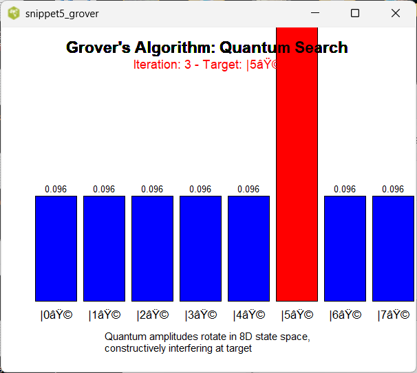
Figure. Simulation entanglement
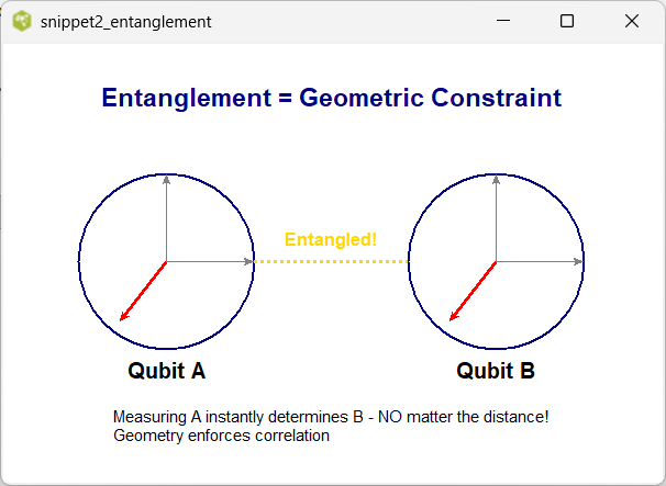
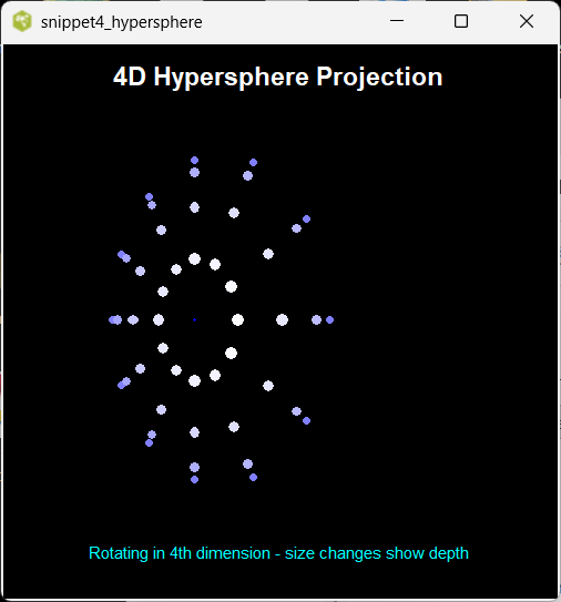
Figure. Simulation Bloch Sphere
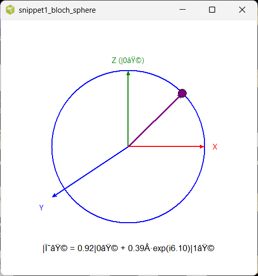
Figure. Simulation stereo
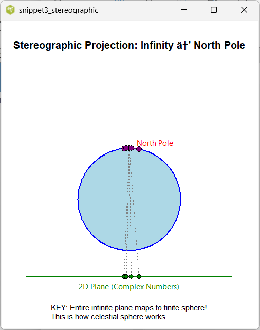
Figure. Simulation paper model
Snippets Concepts Grover Simulation paper model
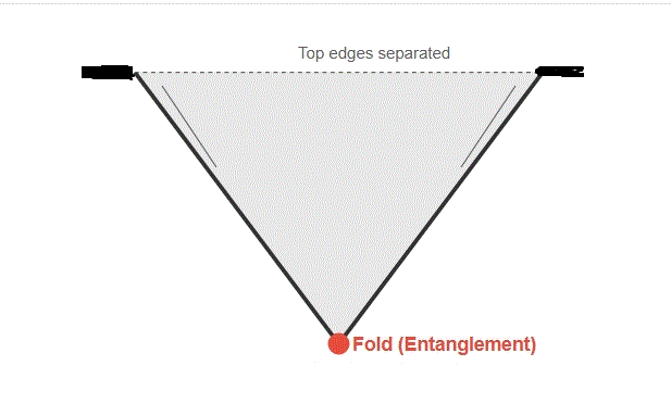
Figure. Model Grid
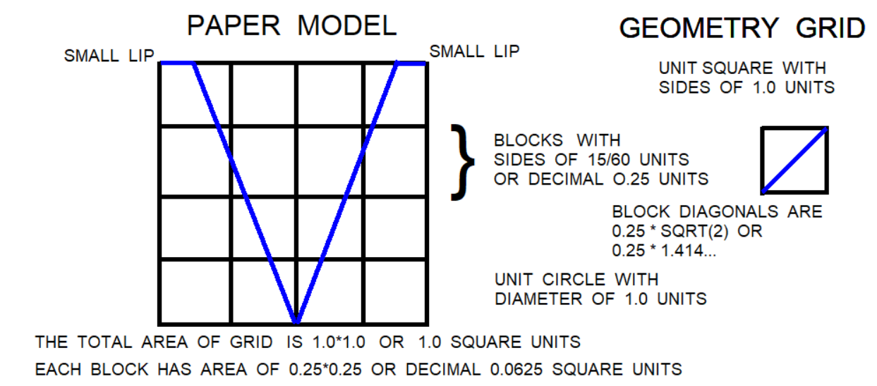
Figure. Orange Tangerine Model
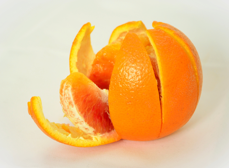
Figure. Analog of Lossless Arrow Hitting Celestial Sphere
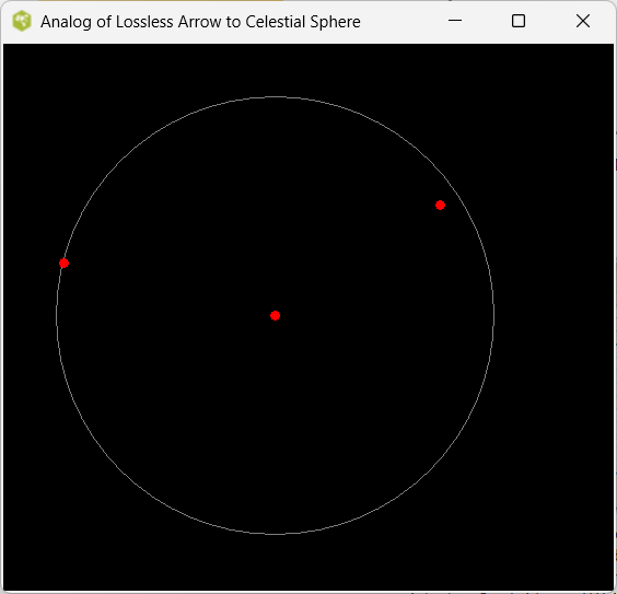
Figure. Mockup on Lossless Arrows Traversing Stellar Neighborhood, Hitting Celestial Sphere
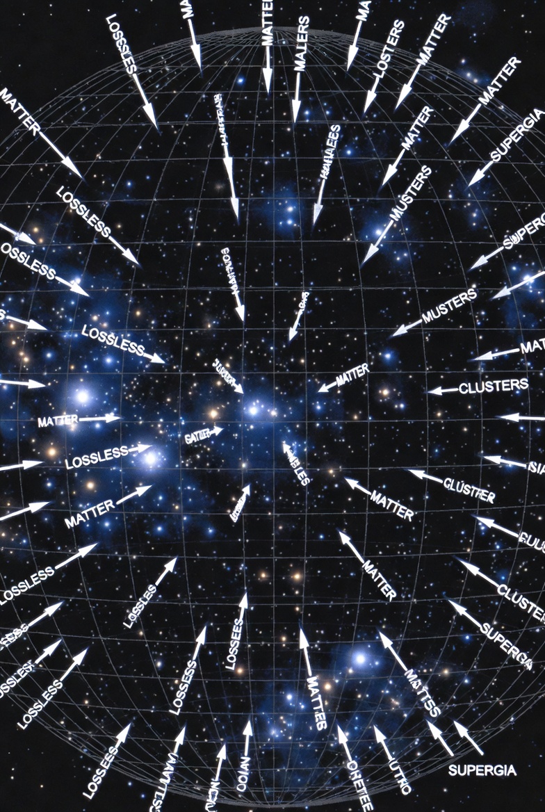
Figure. Rotating Hypersphere
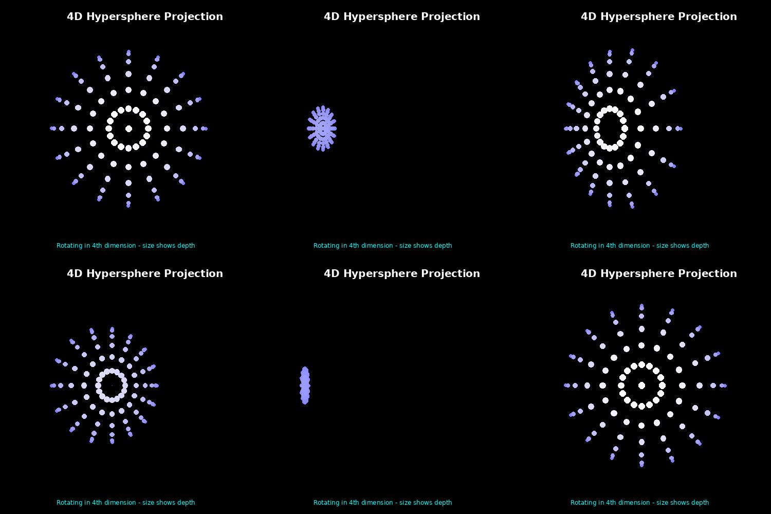
Figure. Hypersphere Simulation on Playground V9
Snippets Concepts Hypersphere Simulation on Playground V9
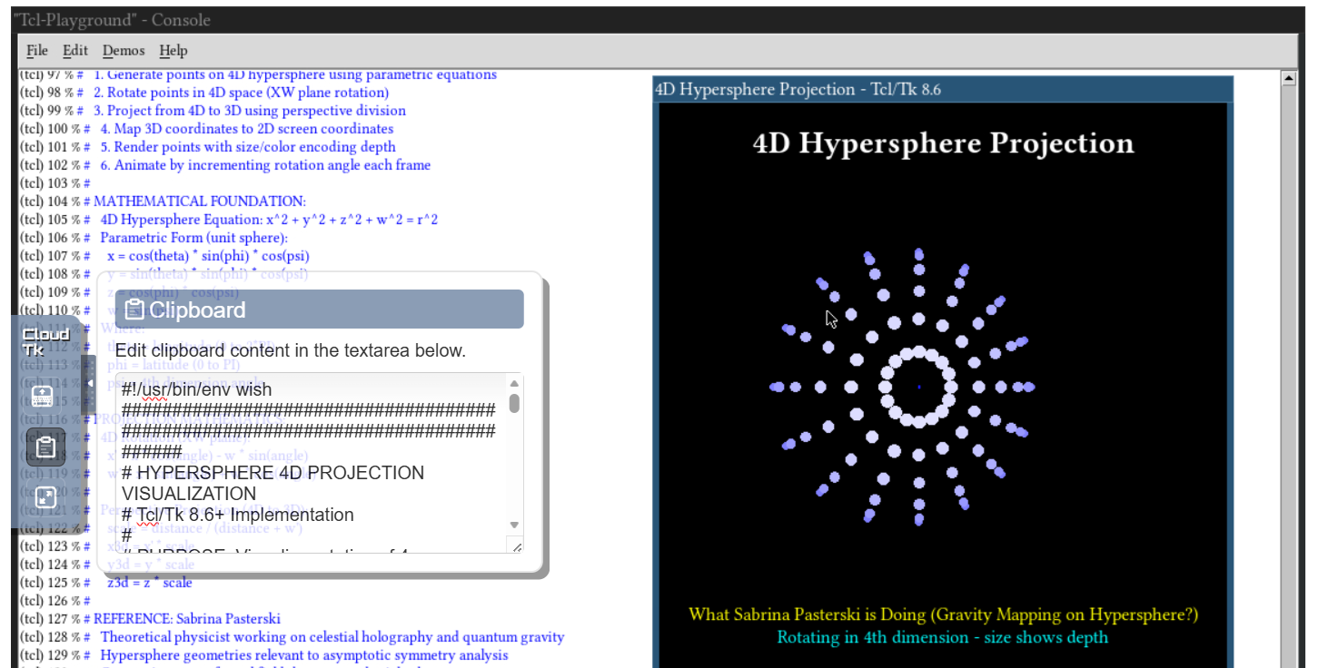
Figure , Parametric Model Mockup Display, Ellipsoid
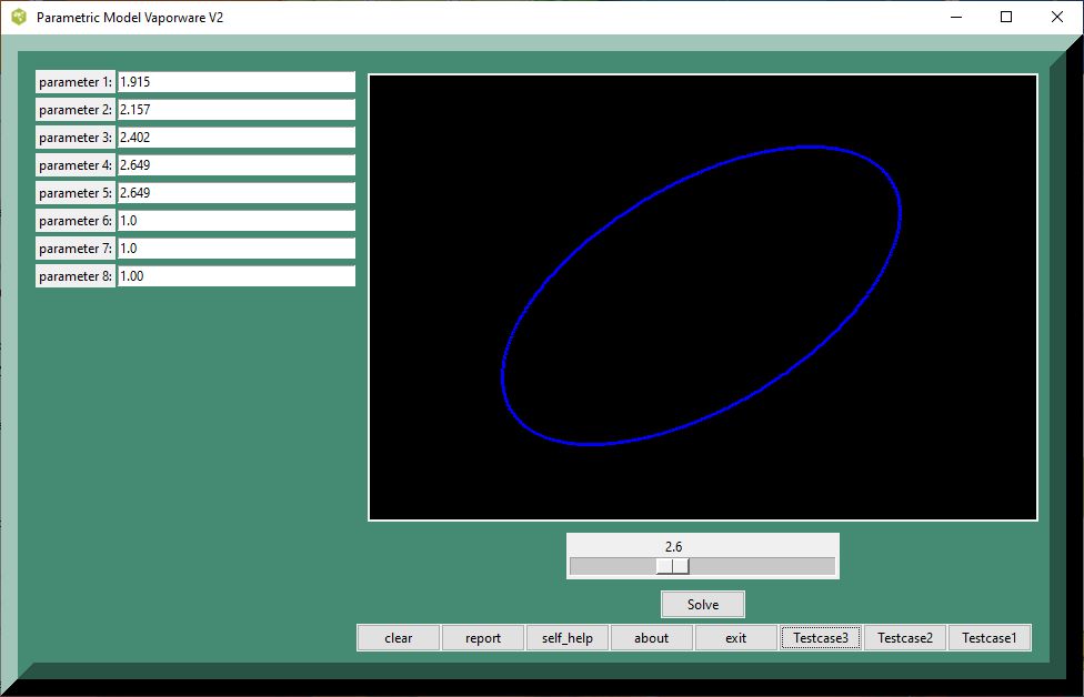
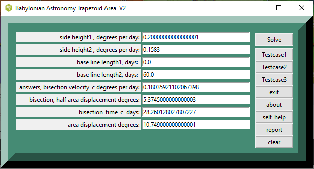
Figure , Sample of plain calculator
Simulation now HyperEllipsoid
Snippets Concepts Hypersphere Simulation now HyperEllipsoid
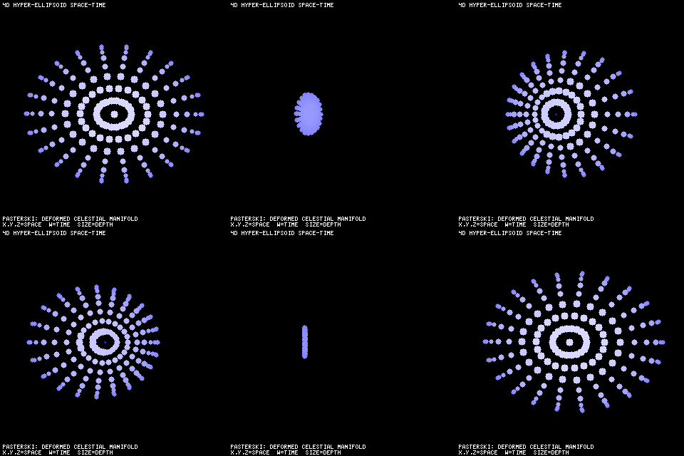
Figure. Hyper-Ellipsoid with Grid on Reflecting Floor
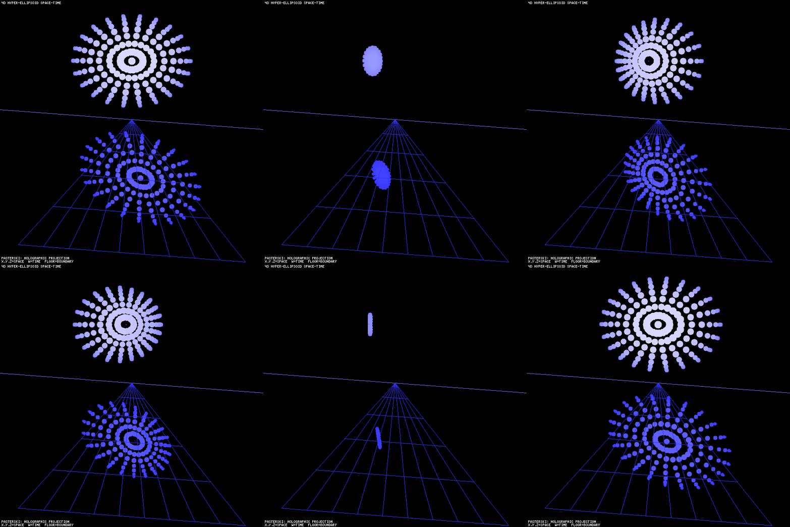
Figure. Composite X_ray all_sky image
Credit. All-sky map from the eROSITA instrument onboard the Spektr-RG (SRG) observatory. An X-ray all-sky image in false color (RGB), showing the sky in soft X-rays at energies from about 0.3 to 2.3 keV (thousands of electron volts).
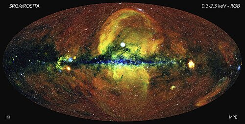
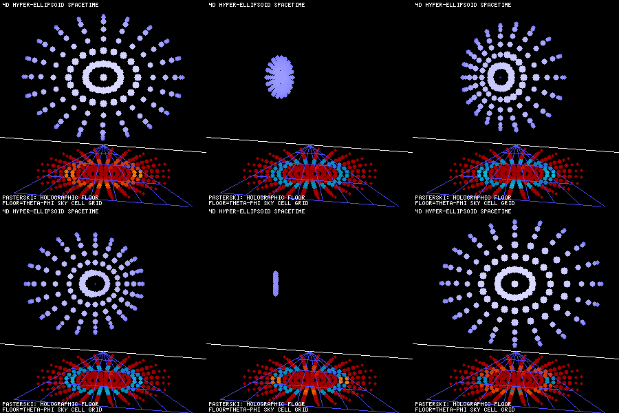
Figure. Composite Reflection,
Testing, concept model of tangerine skin projection into cells by theta and phi from eROSITA X-ray sky image or similar default image. This is an azimuthal equidistant projection; the same projection used in polar maps of Earth and in radio telescope sky maps. Low gif resolution is ~300X300 due saving CS time. These cells have memory storage settings, expect some lag here. Have to check on axis alignments of Hyper-Ellipsoid and its tangerine reflection.
References
- Snippets Physics Concepts Qubits
- Snippets Physics Concepts Feynman
- Snippets Physics Concepts Quantum
- Snippets Physics Concepts Toy
- Snippets Physics Concepts Minimalism
- Zero Handling Workarounds
Note. These Snippets on Theoretical Physics are a set, not stand alones. Recommend read all of the set.
- Celestial Amplitudes: Lecture 1/4 (Sabrina Pasterski)
- Celestial Amplitudes: Lecture 2/4 (Sabrina Pasterski)
- Celestial Amplitudes: Lecture 3/4 (Sabrina Pasterski)
- Celestial Amplitudes: Lecture 4/4 (Sabrina Pasterski)
- Andrea Puhm - Recent advances in celestial holography
- Prof. Sabrina Pasterski lecture– "The Celestial Hologram: From Stargazing to Quantum Gravity and Back”
- A Path To Quantum Gravity , Interview with Prof. Sabrina Pasterski
- Ana-Maria Raclariu lecture , Progress in Celestial Holography
- Lectures on the Infrared Structure of Gravity and Gauge Theory, Andrew Strominger
Appendix Code
Appendix TCL Programs and Scripts
1. Expanded Toy for Demo
convert to strict 7-bit ASCII for Playground V9.
#!/usr/bin/env wish
################################################################################
# HYPERSPHERE 4D PROJECTION VISUALIZATION
# Tcl/Tk 8.6+ Implementation
#
# PURPOSE: Visualize rotation of 4-dimensional hypersphere projected to 3D/2D
# ALGORITHM: Rotate hypersphere in 4D space, project to 3D, then render to 2D
# DISPLAY: Animated canvas showing depth through point size and color
#
# CODING STANDARD: JPL Institutional Coding Standard for C/C++ adapted to Tcl
# - No single-letter variable names (except loop indices in limited scope)
# - Defensive programming with parameter validation
# - Extensive documentation for future maintainers
# - Small, testable modules with single responsibility
# - Explicit error handling
################################################################################
# may have to check strict ASCII for Playground V9
# Compatible with Tcl/Tk 8.6+
# TCL source code follows
# Written for Windows 11 on ActiveState Tcl
# Working on TCL Playground V9, strict ASCII only
# Optimized for collegiate IT lab environments
# Working under TCL version 8.6
# Complex math calculations up to 8 units computer time
# Wait for complete calculations before saving files.
# TCL club, 02/15/2026
# This is a hacker's patch, not rigorously derived.
# appears correct solutions for autotests
# pure ASCII code - no Unicode characters used anywhere
# Approaching =>>> computer time limit on TCL laptop setup.
################################################################################
# MODULE: MATHEMATICAL CONSTANTS
# PURPOSE: Define mathematical constants used throughout program
################################################################################
namespace eval ::constants {
    variable PI 3.14159265358979323846
    variable TWO_PI [expr {2.0 * $PI}]
    variable HALF_PI [expr {$PI / 2.0}]
}

################################################################################
# MODULE: CONFIGURATION PARAMETERS
# PURPOSE: Centralize all tunable parameters for easy maintenance
################################################################################
namespace eval ::config {
    # Display dimensions
    variable canvas_width 500
    variable canvas_height 500

    # Animation parameters
    variable animation_frame_delay_ms 50
    variable total_animation_frames 60

    # Hypersphere geometry
    variable number_of_meridians 16
    variable number_of_parallels 12

    # Projection parameters
    variable projection_distance 2.5
    variable screen_scale_factor 150

    # Visual appearance
    variable point_base_size 3
    variable point_depth_multiplier 3
    variable brightness_base 128
    variable brightness_range 127

    # Colors
    variable background_color "black"
    variable title_color "white"
    variable subtitle_color "yellow"
    variable info_color "cyan"
    variable point_color_base 255  ;# Blue channel always max
}

################################################################################
# MODULE: HYPERSPHERE MATHEMATICS
# PURPOSE: Core mathematical transformations for 4D hypersphere manipulation
################################################################################
namespace eval ::hypersphere {

    ############################################################################
    # FUNCTION: rotate_and_project_4d_to_3d
    # PURPOSE: Rotate point in 4D space and project to 3D using perspective
    # INPUTS:
    #   coord_x - X coordinate in 4D space
    #   coord_y - Y coordinate in 4D space
    #   coord_z - Z coordinate in 4D space
    #   coord_w - W coordinate (4th dimension)
    #   rotation_angle - Angle of rotation in 4D (radians)
    # OUTPUTS: List of {x3d y3d z3d} coordinates in 3D space
    # ALGORITHM:
    #   1. Rotate in XW plane of 4D space
    #   2. Apply perspective projection based on W coordinate
    #   3. Scale remaining coordinates proportionally
    ############################################################################
    proc rotate_and_project_4d_to_3d {coord_x coord_y coord_z coord_w rotation_angle} {
        # Defensive check: ensure angle is numeric
        if {![string is double -strict $rotation_angle]} {
            error "rotation_angle must be numeric, got: $rotation_angle"
        }

        # Calculate rotation trigonometry
        set cosine_angle [expr {cos($rotation_angle)}]
        set sine_angle [expr {sin($rotation_angle)}]

        # Rotate in 4D space (XW plane rotation)
        set rotated_x [expr {$coord_x * $cosine_angle - $coord_w * $sine_angle}]
        set rotated_w [expr {$coord_x * $sine_angle + $coord_w * $cosine_angle}]

        # Perspective projection from 4D to 3D
        # Points further in W dimension appear smaller (perspective)
        set distance $::config::projection_distance
        set perspective_scale [expr {$distance / ($distance + $rotated_w)}]

        # Apply perspective scaling to all 3D coordinates
        set projected_x [expr {$rotated_x * $perspective_scale}]
        set projected_y [expr {$coord_y * $perspective_scale}]
        set projected_z [expr {$coord_z * $perspective_scale}]

        return [list $projected_x $projected_y $projected_z]
    }

    ############################################################################
    # FUNCTION: generate_hypersphere_points
    # PURPOSE: Generate lattice of points on 4D hypersphere surface
    # INPUTS:
    #   rotation_angle - Current rotation angle for animation
    # OUTPUTS: List of point records, each containing:
    #   {screen_x screen_y point_size brightness_value}
    # ALGORITHM:
    #   Uses spherical coordinates extended to 4D:
    #   - Theta: longitude angle (0 to 2*PI)
    #   - Phi: latitude angle (0 to PI)
    #   - W_angle: 4th dimension angle
    ############################################################################
    proc generate_hypersphere_points {rotation_angle} {
        set point_list {}

        set num_meridians $::config::number_of_meridians
        set num_parallels $::config::number_of_parallels

        # Iterate through meridians (longitude lines)
        for {set meridian_index 0} {$meridian_index < $num_meridians} {incr meridian_index} {
            set theta_angle [expr {$meridian_index * $::constants::TWO_PI / $num_meridians}]

            # Iterate through parallels (latitude lines)
            for {set parallel_index 0} {$parallel_index < $num_parallels} {incr parallel_index} {
                set phi_angle [expr {$parallel_index * $::constants::PI / $num_parallels}]

                # 4D hypersphere parametric equations
                # Standard sphere equations extended with W coordinate
                set coord_x [expr {cos($theta_angle) * sin($phi_angle) * cos($rotation_angle)}]
                set coord_y [expr {sin($theta_angle) * sin($phi_angle) * cos($rotation_angle)}]
                set coord_z [expr {cos($phi_angle) * cos($rotation_angle)}]
                set coord_w [expr {sin($rotation_angle)}]

                # Project from 4D to 3D
                lassign [rotate_and_project_4d_to_3d \
                    $coord_x $coord_y $coord_z $coord_w $rotation_angle] \
                    projected_x projected_y projected_z

                # Convert 3D coordinates to 2D screen coordinates
                set screen_x [expr {$::config::canvas_width / 2 + \
                    $projected_x * $::config::screen_scale_factor}]
                set screen_y [expr {$::config::canvas_height / 2 - \
                    $projected_y * $::config::screen_scale_factor}]

                # Point size indicates depth (Z coordinate)
                set point_size [expr {$::config::point_base_size + \
                    $projected_z * $::config::point_depth_multiplier}]

                # Brightness indicates depth (closer = brighter)
                set brightness_value [expr {int($::config::brightness_base + \
                    $projected_z * $::config::brightness_range)}]

                # Clamp brightness to valid range
                if {$brightness_value < 0} {set brightness_value 0}
                if {$brightness_value > 255} {set brightness_value 255}

                # Store point data
                lappend point_list [list $screen_x $screen_y $point_size $brightness_value]
            }
        }

        return $point_list
    }
}

################################################################################
# MODULE: GRAPHICS RENDERING
# PURPOSE: Handle all canvas drawing operations
################################################################################
namespace eval ::graphics {

    ############################################################################
    # FUNCTION: rgb_to_hex_color
    # PURPOSE: Convert RGB values to Tcl/Tk hex color format
    # INPUTS: red_value green_value blue_value (0-255 each)
    # OUTPUTS: Hex color string like "#RRGGBB"
    ############################################################################
    proc rgb_to_hex_color {red_value green_value blue_value} {
        return [format "#%02X%02X%02X" $red_value $green_value $blue_value]
    }

    ############################################################################
    # FUNCTION: sort_points_by_depth
    # PURPOSE: Sort points for painter's algorithm (back-to-front rendering)
    # INPUTS: point_list - List of point records
    # OUTPUTS: Sorted list with furthest points first
    # NOTE: Sorts by point_size as proxy for depth
    ############################################################################
    proc sort_points_by_depth {point_list} {
        return [lsort -real -index 2 $point_list]
    }

    ############################################################################
    # FUNCTION: draw_hypersphere_frame
    # PURPOSE: Render single frame of hypersphere on canvas
    # INPUTS:
    #   canvas_widget - Tk canvas widget path
    #   rotation_angle - Current rotation angle
    ############################################################################
    proc draw_hypersphere_frame {canvas_widget rotation_angle} {
        # Clear previous frame
        $canvas_widget delete all

        # Draw background
        $canvas_widget configure -background $::config::background_color

        # Draw title text
        $canvas_widget create text \
            [expr {$::config::canvas_width / 2}] 20 \
            -text "4D Hypersphere Projection" \
            -fill $::config::title_color \
            -font {Arial 20 bold} \
            -anchor n

        # Draw subtitle (Pasterski reference)
        $canvas_widget create text \
            [expr {$::config::canvas_width / 2}] \
            [expr {$::config::canvas_height - 50}] \
            -text "What Sabrina Pasterski is Doing (Gravity Mapping on Hypersphere?)" \
            -fill $::config::subtitle_color \
            -font {Arial 12} \
            -anchor center

        # Draw info line
        $canvas_widget create text \
            [expr {$::config::canvas_width / 2}] \
            [expr {$::config::canvas_height - 30}] \
            -text "Rotating in 4th dimension - size shows depth" \
            -fill $::config::info_color \
            -font {Arial 12} \
            -anchor center

        # Generate and sort points
        set point_list [::hypersphere::generate_hypersphere_points $rotation_angle]
        set sorted_points [sort_points_by_depth $point_list]

        # Draw each point
        foreach point_record $sorted_points {
            lassign $point_record screen_x screen_y point_size brightness_value

            # Only draw points with positive size
            if {$point_size > 0.5} {
                # Calculate point color (blue gradient based on depth)
                set point_color [rgb_to_hex_color \
                    $brightness_value \
                    $brightness_value \
                    $::config::point_color_base]

                # Calculate bounding box for oval
                set bbox_x1 [expr {$screen_x - $point_size}]
                set bbox_y1 [expr {$screen_y - $point_size}]
                set bbox_x2 [expr {$screen_x + $point_size}]
                set bbox_y2 [expr {$screen_y + $point_size}]

                # Draw point as filled oval
                $canvas_widget create oval \
                    $bbox_x1 $bbox_y1 $bbox_x2 $bbox_y2 \
                    -fill $point_color \
                    -outline $point_color
            }
        }
    }
}

################################################################################
# MODULE: ANIMATION CONTROL
# PURPOSE: Manage animation loop and frame timing
################################################################################
namespace eval ::animation {
    variable current_frame_number 0
    variable animation_running 0
    variable animation_id ""

    ############################################################################
    # FUNCTION: calculate_rotation_angle
    # PURPOSE: Calculate rotation angle for given frame number
    # INPUTS: frame_number - Current frame in animation sequence
    # OUTPUTS: Rotation angle in radians (0 to 2*PI)
    ############################################################################
    proc calculate_rotation_angle {frame_number} {
        set total_frames $::config::total_animation_frames
        return [expr {$frame_number * $::constants::TWO_PI / $total_frames}]
    }

    ############################################################################
    # FUNCTION: animate_next_frame
    # PURPOSE: Draw next frame and schedule subsequent frame
    # INPUTS: canvas_widget - Tk canvas widget path
    ############################################################################
    proc animate_next_frame {canvas_widget} {
        variable current_frame_number
        variable animation_running
        variable animation_id

        if {!$animation_running} {
            return
        }

        # Calculate rotation angle for this frame
        set rotation_angle [calculate_rotation_angle $current_frame_number]

        # Draw frame
        ::graphics::draw_hypersphere_frame $canvas_widget $rotation_angle

        # Advance to next frame (loop back to 0 after last frame)
        incr current_frame_number
        if {$current_frame_number >= $::config::total_animation_frames} {
            set current_frame_number 0
        }

        # Schedule next frame
        set animation_id [after $::config::animation_frame_delay_ms \
            [list ::animation::animate_next_frame $canvas_widget]]
    }

    ############################################################################
    # FUNCTION: start_animation
    # PURPOSE: Begin animation loop
    ############################################################################
    proc start_animation {canvas_widget} {
        variable animation_running
        variable current_frame_number

        set animation_running 1
        set current_frame_number 0
        animate_next_frame $canvas_widget
    }

    ############################################################################
    # FUNCTION: stop_animation
    # PURPOSE: Halt animation loop
    ############################################################################
    proc stop_animation {} {
        variable animation_running
        variable animation_id

        set animation_running 0
        if {$animation_id ne ""} {
            after cancel $animation_id
            set animation_id ""
        }
    }
}

################################################################################
# MODULE: USER INTERFACE
# PURPOSE: Create and configure GUI elements
################################################################################
namespace eval ::gui {

    ############################################################################
    # FUNCTION: create_main_window
    # PURPOSE: Build complete user interface
    # OUTPUTS: Canvas widget path for animation
    ############################################################################
    proc create_main_window {} {
        # Configure main window
        wm title . "4D Hypersphere Projection - Tcl/Tk 8.6"
        wm geometry . "${::config::canvas_width}x[expr {$::config::canvas_height + 60}]"
        wm resizable . 0 0

        # Create canvas for drawing
        set canvas_widget [canvas .canvas \
            -width $::config::canvas_width \
            -height $::config::canvas_height \
            -background $::config::background_color \
            -highlightthickness 0]

        pack $canvas_widget -side top -fill both -expand 1

        # Create control frame
        set control_frame [frame .controls -relief raised -borderwidth 2]
        pack $control_frame -side bottom -fill x

        # Create control buttons
        button $control_frame.start \
            -text "Start Animation" \
            -command [list ::animation::start_animation $canvas_widget]

        button $control_frame.stop \
            -text "Stop Animation" \
            -command ::animation::stop_animation

        button $control_frame.quit \
            -text "Quit" \
            -command exit

        pack $control_frame.start $control_frame.stop $control_frame.quit \
            -side left -padx 5 -pady 5

        return $canvas_widget
    }
}

################################################################################
# MODULE: MAIN PROGRAM
# PURPOSE: Entry point and initialization
################################################################################

############################################################################
# FUNCTION: main
# PURPOSE: Initialize application and start event loop
############################################################################
proc main {} {
    # Create user interface
    set canvas_widget [::gui::create_main_window]

    # Draw initial frame (frame 0)
    ::graphics::draw_hypersphere_frame $canvas_widget 0.0

    # Auto-start animation
    after 500 [list ::animation::start_animation $canvas_widget]

    # Note: Tk event loop starts automatically with wish interpreter
}

################################################################################
# DOCUMENTATION SECTION: SNIPPETS CONCEPTS EFFECTS
################################################################################
# CONCEPT: 4D Hypersphere
#   A hypersphere is the 4-dimensional analogue of a sphere
#   Just as a sphere is the set of all points equidistant from a center in 3D,
#   a hypersphere is the set of all points equidistant from a center in 4D
#
# EFFECT: Rotation Visualization
#   By rotating the hypersphere in 4D space and projecting to 3D, then 2D,
#   we can visualize aspects of 4-dimensional geometry
#   Points appear to expand/contract and change brightness based on their
#   position in the 4th dimension
#
# EFFECT: Perspective Projection
#   Points further away in the W dimension (4th dimension) appear smaller
#   This mimics how 3D perspective works when projecting to 2D screens
#
# EFFECT: Depth Cueing
#   Point size and brightness encode depth information
#   Larger, brighter points are "closer" to the viewer in 3D projection
#   This helps the human visual system interpret the 3D structure
################################################################################

################################################################################
# DOCUMENTATION SECTION: SNIPPETS CONCEPTS HYPERSPHERE SIMULATION
################################################################################
# SIMULATION ALGORITHM:
#   1. Generate points on 4D hypersphere using parametric equations
#   2. Rotate points in 4D space (XW plane rotation)
#   3. Project from 4D to 3D using perspective division
#   4. Map 3D coordinates to 2D screen coordinates
#   5. Render points with size/color encoding depth
#   6. Animate by incrementing rotation angle each frame
#
# MATHEMATICAL FOUNDATION:
#   4D Hypersphere Equation: x^2 + y^2 + z^2 + w^2 = r^2
#   Parametric Form (unit sphere):
#     x = cos(theta) * sin(phi) * cos(psi)
#     y = sin(theta) * sin(phi) * cos(psi)
#     z = cos(phi) * cos(psi)
#     w = sin(psi)
#   Where:
#     theta = longitude (0 to 2*PI)
#     phi = latitude (0 to PI)
#     psi = 4th dimension angle
#
# PROJECTION MATHEMATICS:
#   4D Rotation (XW plane):
#     x' = x * cos(angle) - w * sin(angle)
#     w' = x * sin(angle) + w * cos(angle)
#
#   Perspective Projection (4D to 3D):
#     scale = distance / (distance + w')
#     x3d = x' * scale
#     y3d = y * scale
#     z3d = z * scale
#
# REFERENCE: Sabrina Pasterski
#   Theoretical physicist working on celestial holography and quantum gravity
#   Hypersphere geometries relevant to asymptotic symmetry analysis
#   Connection to conformal field theory on celestial sphere
################################################################################

# Execute main program
main

# End of hypersphere_4d_projection.tcl
Output from ActiveState
Appears correct for limited iterations.
Added tests from ActiveState Version
Approaching =>>> computer time limit in this TCL configuration. this list-based simulation becomes very slow (2ⁿ memory/time) on laptop.
Toy Solver
# Relativistic momentum calculation V2
# may have to check strict ASCII for Playground V9
# Compatible with Tcl/Tk 8.6+
# TCL source code follows
# Written for Windows 11 on ActiveState Tcl
# Working on TCL Playground V9, strict ASCII only
# Optimized for collegiate IT lab environments
# Working under TCL version 8.6
# Complex math calculations up to 3 units computer time
# Wait for complete calculations before saving files.
# TCL club, 02/24/2026
# This is a hacker's patch, not rigorously derived.
# appears correct solutions
# pure ASCII code - no Unicode characters used anywhere
# May Approach =>>> computer time limit on TCL laptop setup.

# Taciturn formula from math textbooks
# Momentum p = gamma * m * v, where gamma = 1 / sqrt(1 - v^2/c^2)

# Pseudocode style in plain English
# relativistic_momentum = relativistic_factor * rest_mass * velocity
# where relativistic_factor = 1 / square_root(1 - (velocity^2 / speed_of_light^2))
# Relativistic momentum calculation

# Switching to human readable variables in Tcl
# All speeds must be in the same units (e.g. m/s); speed_of_light ≈ 299792458 m/s

set rest_mass_kg          9.1093837e-31     ;# example: electron rest mass
set velocity_m_per_s      2.5e8              ;# example: 0.833 c
set speed_of_light_m_per_s 299792458.0

# Step 1: Compute the relativistic factor (gamma)
set velocity_squared_over_c_squared [expr {pow($velocity_m_per_s, 2) / pow($speed_of_light_m_per_s, 2)}]
set relativistic_factor [expr {1.0 / sqrt(1.0 - $velocity_squared_over_c_squared)}]

# Step 2: Compute relativistic momentum
set relativistic_momentum_kg_m_per_s [expr {$relativistic_factor * $rest_mass_kg * $velocity_m_per_s}]

puts "Rest mass:                  [format %.3e $rest_mass_kg] kg"
puts "Velocity:                   [format %.3e $velocity_m_per_s] m/s"
puts "Relativistic factor (gamma): [format %.4f $relativistic_factor]"
puts "Relativistic momentum:      [format %.4e $relativistic_momentum_kg_m_per_s] kg m/s"
Output from ActiveState
Rest mass:                  9.109e-31 kg
Velocity:                   2.500e+08 m/s
Relativistic factor (gamma): 1.8119
Relativistic momentum:      4.1264e-22 kg m/s
(bin) 1 %
This is a draft, still debugging on Playground V9. convert to strict 7-bit ASCII for Playground V9.
Output from Playground V9
(tcl) 8 % # Switching to human readable variables in Tcl
(tcl) 9 % # All speeds must be in the same units (e.g. m/s); speed_of_light ≈ 299792458 m/s
(tcl) 10 %
(tcl) 10 % set rest_mass_kg          9.1093837e-31     ;# example: electron rest mass
9.1093837e-31
(tcl) 11 % set velocity_m_per_s      2.5e8              ;# example: 0.833 c
2.5e8
(tcl) 12 % set speed_of_light_m_per_s 299792458.0
299792458.0
(tcl) 13 %
(tcl) 13 % # Step 1: Compute the relativistic factor (gamma)
(tcl) 14 % set velocity_squared_over_c_squared [expr {pow($velocity_m_per_s, 2) / pow($speed_of_light_m_per_s, 2)}]
0.6954062850335115
(tcl) 15 % set relativistic_factor [expr {1.0 / sqrt(1.0 - $velocity_squared_over_c_squared)}]
1.8119221375144938
(tcl) 16 %
(tcl) 16 % # Step 2: Compute relativistic momentum
(tcl) 17 % set relativistic_momentum_kg_m_per_s [expr {$relativistic_factor * $rest_mass_kg * $velocity_m_per_s}]
4.1263734962859223e-22
(tcl) 18 %
(tcl) 18 % puts "Rest mass:                  [format %.3e $rest_mass_kg] kg"
Rest mass:                  9.109e-31 kg
(tcl) 19 % puts "Velocity:                   [format %.3e $velocity_m_per_s] m/s"
Velocity:                   2.500e+08 m/s
(tcl) 20 % puts "Relativistic factor (gamma): [format %.4f $relativistic_factor]"
Relativistic factor (gamma): 1.8119
(tcl) 21 % puts "Relativistic momentum:      [format %.4e $relativistic_momentum_kg_m_per_s] kg m/s"
Relativistic momentum:      4.1264e-22 kg m/s
(tcl) 22 %
Output from ActiveState
Table on Comparison for Hyper-Ellipsoid Simulation, Python style Pseudocode vs Tcl style Pseudocode equivalent
Columns: index_number, Python style pseudocode, Tcl style equivalent, pseudocode_comment, quibble_notes.
| index_number | Python style pseudocode | Tcl style equivalent | pseudocode_comment | quibble_notes |
|---|---|---|---|---|
| 1 | import numpy as np | # require Tcllib math or external N‑D package | Import numerical library for randoms and vector ops | Pure NumPy not available in Tcl core, use rand(), mathfuncs, or external libs |
| 2 | a,b,c,d = 1.0,0.95,0.90,1.10 | set a 1.0; set b 0.95; set c 0.90; set d 1.10 | Semi‑axes of 4D hyper‑ellipsoid, encode anisotropy | Values represent gravitational deformation, tweakable parameters |
| 3 | N = 10000 | set N 10000 | Number of surface sample points (information nodes/pores) | N may be reduced on slow laptops for timing and plots |
| 4 | theta1 = rand(0,pi,N) | set theta1L list; for {set k 0} {$k<$N} {incr k} {lappend theta1L expr {rand()acos(-1)}} | Sample polar angle theta1 uniformly on 0,pi | Tcl uses acos(-1) for pi; list comprehension done by loop |
| 5 | theta2 = rand(0,pi,N) | set theta2L list; for {set k 0} {$k<$N} {incr k} {lappend theta2L expr {rand()acos(-1)}} | Second polar angle theta2 for 4D sphere coords | Can reuse loop or share RNG seed for reproducibility |
| 6 | phi = rand(0,2pi,N) | set phiL list; set twopi expr {2.0acos(-1)}; for {set k 0} {$k<$N} {incr k} {lappend phiL expr {rand()$twopi}} | Azimuthal angle on 0,2pi | Watch numeric overflow if twopi computed repeatedly inside loop |
| 7 | x1 = asin(theta1)sin(theta2)cos(phi) | # in loop: set x1 expr {$asin($t1)sin($t2)cos($p)} | First coordinate of hyper‑ellipsoid surface point | Implement inside single loop over k reading list elements |
| 8 | x2 = bsin(theta1)sin(theta2)sin(phi) | # in loop: set x2 expr {$bsin($t1)sin($t2)sin($p)} | Second coordinate, scaled by semi‑axis b | Keep expr arguments simple, avoid nested list commands |
| 9 | x3 = csin(theta1)cos(theta2) | # in loop: set x3 expr {$csin($t1)cos($t2)} | Third coordinate, uses cos(theta2) | c < 1.0 flattens along x3 direction |
| 10 | x4 = dcos(theta1) | # in loop: set x4 expr {$dcos($t1)} | Fourth coordinate, pure cos(theta1) scaling | d slightly > 1.0 gives elongation in x4 axis |
| 11 | r3 = sqrt(x12 + x22 + x3**2) | set r3 expr {sqrt($x1$x1 + $x2$x2 + $x3$x3)} | Radius in 3D after dropping x4 for projection | Guard against r3==0.0 to avoid division warnings |
| 12 | theta_cel = arccos(x3/r3) | set theta_cel expr {acos($x3/$r3)} | Celestial polar angle on projected S^2 | Domain of acos requires -1.0<=x3/r3<=1.0 numerically |
| 13 | phi_cel = arctan2(x2,x1) | set phi_cel expr {atan2($x2,$x1)} | Celestial azimuthal angle on projected S^2 | atan2 argument order in Tcl is atan2(y,x) same as Python |
| 14 | plot(theta_cel,phi_cel) | # delegate to Tk canvas, plot points (theta_cel,phi_cel) | Visualize pore density on 2D celestial sphere | Can use polar or Cartesian canvas mapping for display |
| 15 | # density encodes bulk curvature | # comment: bin projected points into histogram | Pore density pattern encodes curvature / information flux heuristically | Tutorial visualization only, not full GR or QFT simulation |
| 16 | # TODO: extend to time slices | # comment: later add loop over time index t | Future work hook for rotating or evolving hyper‑ellipsoid | Keeps snippet under 30 lines, extensions possible |
Pseudocode Comparison
gravity_sim_pseudocode.csv:

text
index_number,Python style pseudocode,Tcl style equivalent,pseudocode_comment,quibble_notes
1,"# Gravitational wave perturbation (+ polarization)","# Gravitational wave perturbation (+ polarization)","Header comment for GW + polarization case","Purely descriptive, no executable effect"
2,"t = np.linspace(0, 10, 1000)","set tL [list]; set t0 0.0; set t1 10.0; set Nt 1000","Declare time array from 0 to 10 with Nt samples","Tcl uses explicit loop or helper proc to fill tL"
3,"# time array","# time array","Comment that t is the simulation time grid","Could store dt instead of full list for some uses"
4,"h_plus = 1e-4 * np.sin(2 * np.pi * 0.5 * t)","set hL [list]","Define GW strain h_plus as small sinusoid","Need later loop to append per-time h values"
5,"# strain amplitude","# strain amplitude","Note that h_plus is dimensionless strain","Amplitude 1e-4 is exaggerated vs. realistic LIGO"
6,"for each t in time array:","for {set i 0} {$i < $Nt} {incr i} {","Loop over time grid indices","Pseudocode loop; body filled in next rows"
7,"    h = 1e-4 * sin(2*pi*0.5*t)","  set ti [expr {$t0 + double($i)*($t1-$t0)/($Nt-1)}]","Compute current time ti for index i","Linear spacing between t0 and t1"
8,"    h_plus[i] = h","  set h [expr {1.0e-4 * sin(2.0*acos(-1)*0.5*$ti)}]","Evaluate sinusoidal strain at ti","acos(-1) used as pi in Tcl expr"
9,"    # store h_plus[i]","  lappend tL $ti; lappend hL $h","Append time and strain to lists","Mimics NumPy vectorization with manual list build"
10,"end for","}","End time loop over GW strain","Closing brace only, no extra action"
11,"a_t = 1.0 + h_plus","# inside loop: set a_t [expr {1.0 + $h}]","x1 semi-axis stretches with the wave","In Tcl, a_t is instantaneous value, not full array"
12,"b_t = 1.0 - h_plus","# inside loop: set b_t [expr {1.0 - $h}]","x2 semi-axis compresses with opposite sign","Same instantaneous semantics as a_t"
13,"# x3, x4 axes unaffected","# x3, x4 axes unaffected by + polarization","Comment: other axes unchanged for + mode","Cross and higher modes omitted here"
14,"a_t_list.append(a_t)","  lappend aL $a_t","Store time series of a_t semi-axis","Requires aL initialized before loop"
15,"b_t_list.append(b_t)","  lappend bL $b_t","Store time series of b_t semi-axis","Requires bL initialized before loop"
16,"# This is LIGO mechanism","# This is LIGO mechanism","Comment: differential arm stretching is detector signal","Extremely simplified description of interferometer readout"
17,"# metric oscillates, axes stretch/contract","# metric oscillates, axes stretch/contract","Summarizes spacetime interpretation of GW strain","Leaves out tensor notation and full GR details"
Table‑driven pseudocode with comments
For hypersphere / hyper‑ellipsoid
| Step | Pseudocode line | Comment |
|---|---|---|
| 1 | SET N = 10000 | Number of sample points on hypersphere surface |
| 2 | SET (a,b,c,d) = (1.0,0.95,0.90,1.10) | Semi‑axes, encode anisotropy / deformation |
| 3 | FOR k FROM 1 TO N | Loop over sample index k |
| 4 | DRAW theta1, theta2, phi AT RANDOM | Random angles on 4‑sphere |
| 5 | COMPUTE (x1,x2,x3,x4) ON HYPER‑ELLIPSOID | Scale 4D point by (a,b,c,d) |
| 6 | PROJECT (x1,x2,x3) TO CELESTIAL ANGLES | Compute theta_cel, phi_cel |
| 7 | RECORD projected point | Store pore / information node |
| 8 | END FOR | End sampling loop |
Example inline pseudocode block
Use an inline, keyword‑capitalized style plus a short explanation paragraph.
text
PSEUDOCODE:
START
  GET user input
  IF user input is valid
    CALL process user input
    DISPLAY processed user input
  ELSE
    DISPLAY invalid input message
  END IF
END
Pseudocode for Gravity Wave Simulation
| index_number | Python style pseudocode | Tcl style equivalent | pseudocode_comment | quibble_notes |
|---|---|---|---|---|
| 1 | import numpy as np | package require Tcl | Initialize environment and imports. | Standard setup for numerical work; use lists in Tcl. |
| 2 | t = np.linspace(0, 10, 1000) | set tL {}; set t0 0.0; set t1 10.0; set Nt 1000; for {set i 0} {$i < $Nt} {incr i} { set ti expr {$t0 + double($i)($t1-$t0)/($Nt-1)}; lappend tL $ti } | Create time array over with 1000 points. | Linear spacing; Tcl uses explicit loop for list building. |
| 3 | h_plus = 1e-4 * np.sin(2 * np.pi * 0.5 * t) | set hL {}; foreach ti $tL { set h expr {1.0e-4 * sin(2.0acos(-1)0.5$ti)}; lappend hL $h } | Define + polarization strain: small sinusoidal amplitude 10^-4, freq 0.5 Hz. | Strain h(t) models metric oscillation; sin(ωt) form common in GW sims. |
| 4 | a_t = 1.0 + h_plus | set aL {}; foreach h $hL { set a_t expr {1.0 + $h}; lappend aL $a_t } | Perturb semi-axis a: stretch along one direction. | + polarization effect; a increases with positive strain. |
| 5 | b_t = 1.0 - h_plus | set bL {}; foreach h $hL { set b_t expr {1.0 - $h}; lappend bL $b_t } | Perturb semi-axis b: compress orthogonally. | Opposite sign for quadrupole nature of GWs. |
| 6 | # c_t = 1.0; d_t = 1.0 | set c_t 1.0; set d_t 1.0 | x3 and x4 axes unaffected in + polarization. | Simplified model; cross polarization would affect others. |
| 7 | # Store or plot: e.g., plt.plot(t, a_t - 1.0) | # e.g., canvas plot of (a_t - 1.0) vs ti | Track differential strain da = a_t - 1.0. | Observable in simulation; mimics arm length change in interferometers. |
| 8 | # Integrate over time for cumulative effect | # Accumulate phase or memory effect if needed | Consider permanent displacement (memory). | Advanced: nonlinear memory from GW bursts not in linear approx here. |
| 9 | # Project perturbed ellipsoid to celestial sphere | # Use Tcl projection: drop x4, normalize (x1,x2,x3) to angles | Map perturbed 4D surface to 2D boundary. | Ties to Pasterski celestial holography: GW imprints on null infinity sphere. |
| 10 | # Analyze pore/distortion count on projected rind | # Count features in 2D map after perturbation | Quantify information nodes or boundary changes. | Analog to tangerine pores; distortion reveals anomaly approach. |
"1","import numpy as np","package require Tcl","Initialize environment and imports.","Standard setup; Tcl uses lists instead of numpy arrays."
"2","t = np.linspace(0,10,1000)","set tL {};set t0 0.0;set t1 10.0;set Nt 1000;for {set i 0} {$i<$Nt} {incr i} {set ti [expr {$t0+double($i)($t1-$t0)/($Nt-1)}];lappend tL $ti}","Create evenly spaced time array over [0,10] with 1000 points.","Tcl has no built-in linspace; explicit loop is standard."
"3","h_plus = 1e-4np.sin(2np.pi0.5t)","set pi [expr {acos(-1.0)}];set hL {};foreach ti $tL {lappend hL [expr {1e-4sin(2*$pi0.5$ti)}]}","Define + polarization strain h₊(t): amplitude 10⁻⁴, frequency 0.5 Hz.","Toy frequency; real GW events often 10–1000 Hz range."
"4","a_t = 1.0 + h_plus","set aL {};foreach h $hL {lappend aL [expr {1.0+$h}]}","Perturb semi-axis a: stretch in + polarization direction.","Quadrupole pattern: one axis expands when orthogonal compresses."
"5","b_t = 1.0 - h_plus","set bL {};foreach h $hL {lappend bL [expr {1.0-$h}]}","Perturb semi-axis b: compress orthogonally.","Opposite sign reflects + polarization signature."
"6","","set c_t 1.0;set d_t 1.0","x3 and x4 axes remain unperturbed in + polarization.","Cross (+) polarization affects only two orthogonal axes."
"7","# Example: differential strain da = a_t - 1.0","# set daL {};foreach a $aL {lappend daL [expr {$a-1.0}]}","Track observable strain difference da(t).","Mimics LIGO arm-length change detection."
"8","# Optional: plot or export (t, h_plus, da)","# Use canvas or write to file for visualization","Visualize perturbation over time.","Useful for debugging or educational demo in TCL."
"9","# Project perturbed 4D ellipsoid to 2D celestial boundary","# Normalize (a_t,b_t,1.0,1.0) → spherical angles θ,φ","Map GW-distorted hyper-ellipsoid to celestial sphere.","Links to Pasterski celestial holography: GW memory imprints boundary."
"10","# Count/measure “pores” or features on projected 2D rind","# After projection, tally distortion nodes or curvature gradients","Quantify boundary information change due to GW.","Tangerine analog: more/stretched pores signal anomaly approach."
Credit to the eROSITA instrument onboard the Spektr-RG (SRG) observatory.
Page Is Under Development
This page is under development. Comments are welcome, but please load any comments in the comments section at the bottom of the page. Please include your wiki MONIKER and date in your comment with the same courtesy that I will give you. Aside from your courtesy, your wiki MONIKER and date as a signature and minimal good faith of any internet post are the rules of this TCL-WIKI. Its very hard to reply reasonably without some background of the correspondent on his WIKI bio page. Thanks, gold 5Jan2026
gold 2/9/2026. Added categories, so can find message in Wiki.
Hidden Comments Section
Program Change Log
gold 2/3/2025. Testing, encountered initial difficulty in saving work? Long code blocks with or unmatched wiki markup can sometimes confuse the Tcl Wiki formatting engine, especially if fences are not balanced or a line begins with markup it treats specially.
gold 2/14/2026. Added Automatic Dump of Examples, Using ActiveState.
gold 2/14/2026. convert to strict 7-bit ASCII for Playground V9. reporting error at bottom. program should run to completion with automatic test suite.
gold 2/14/2026.
two separate bugs fixed on 1-2 iterations, but solution looks rough here:

The oracle is flipping the wrong component.

The diffusion step is mathematically fine, but with the wrong oracle it cancels out and leaves the state uniform.
gold 2/14/2026. convert to strict 7-bit ASCII for Playground V9. variables need to be human readable and very explanatory. avoid variables with single letter names. Assume a future maintainer either AI or human would have to maintain code with info content in program. the program is working the numbers correctly . so minimal changes.
gold 2/19/2026. Python version with floor compiled on laptop. Image is clipping on floor on bottom of image about half disk. Like to see whole disk on bottom reflection. maybe increase image size by 200%. just a hacker's estimate. You may disagree.
gold 2/20/2026. With much help, I have gotten so far with my tangerine model of space-time. I study concepts of “peeling space-time hyper-ellipsoid and laying the gravity information in the ‘peels’ flat of the reflection floor.” Would a Koch roughness on the skin serve here, or is that a false track? Image on the floor would look like 8-sectioned tangerine peels — forgive the ASCII. {} {} {} {} {} {} {} {}
Please place any comments here with your wiki MONIKER and date, Thanks.gold 1/30/2026
Note. Testing computer methods and computer programs, maybe wrong numbers.
| Category Numerical Analysis | Category Toys | Category Calculator | Category Mathematics | Category Example | Toys and Games | Category Games | Category Application | Category GUI |