Tcl based signal processing fundamentals: Additive Wave Synthesis

started by Theo Verelst

When wanting to examplify what frequency varied sine waves have as a spectrum, because that's important while analysing many types of measured or synthesized digital signal, for which tcl is also used, the page on that subject got a bit full. I though some of these very fundamental sujects deserve a place amoung the many pages about these important signal processing subjects, which can be successfully and interestingly programmed in tcl. In fact I prefer to use Tk, too, because it is one of the powers of tcl/tk to be a great interactive program development environment with great scientific value as such. Not many computer languages are really suitable for interactive scientific development , which is probably the main driving force for improvements in computer programming (apart from all kinds of (un-) human, political and 'imperialistic' considerations, and un-technical logics).

Waves can in tcl be natually represented in sampled form as lists. That means that when a wave like a sine is chopped in pieces, or neater put: approximated in x (or time) and y axis sense by rounding it to points on a rectangular grid (like on uses in mathematics school sheets), those point can be stored in order (from left to right) by putting the approximate values in a tcl list of values.

A sine wave is a special repetitive wave pattern, because our ears perceive it has having only one frequency, so it is per definition the most 'dull' or harmonics-poor wave. It isn't hard to make a list with sine values for one sine wave in tcl. Lets say we want ten values for one full wave, we'd write:

set pi 3.1415926535
for {set i 0} {$i < 10} {incr i} {
    puts [expr {sin(2.0*$pi*$i/10)}]
}

Later on we'll put these points in a tcl list, in order, to reuse them, instead of just listing the sine values on the console. To graphically make clear what our wave looks like, we can plot the values in a graph, like so:

# First, a few condensed procs to do make a canvas and draw points on it
# It's always handy to be able to change to which canvas we use
set mc .c
# make the simplest decent canvas
pack [canvas $mc] -expand y -fill both
# define the point drawing procedure
proc plotpoint {x y {size 3} {colour black} {tag p}} {
    global mc;
    $mc create oval \
        [expr {$x-$size/2}] [expr {$y-$size/2}] \
        [expr {$x+$size/2}] [expr {$y+$size/2}] \
        -outline $colour -fill $colour -tag $tag
}
# now the same as above, except scaled and as graphics points
set pi 3.1415926535
set yscale 100
set xscale 20
for {set i 0} {$i < 10} {incr i} {
    plotpoint [expr {10+$i*$xscale}] [expr {150-$yscale*sin(2.0*$pi*$i/10)}]
}

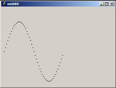
This gives an impression of a sine wave, though it's not all to clear unless we use more points to approximate this important tcl function:

set xp 50;                   # number of X coordinates, or points
set xscale [expr {200/$xp}]; # horizontal space per point in canvas pixels
$mc del p;                   # delete all graphs with tag 'p' from the canvas first
for {set i 0} {$i < $xp} {incr i} {
    plotpoint [expr {10+$i*$xscale}] [expr {150-$yscale*sin(2.0*$pi*$i/$xp)}]
}

The resulting graph

Instead of plotting the sine wave points one by one straight away in the loop, we can first keep them stored in a tcl list, and make a procedure to automatically draw then from a list:

# list the points for one waveform
set wave1 {};    # empty list
for {set i 0} {$i < 100} {incr i} {
    # append each of the 100 points to the list
    lappend wave1 [expr {sin(2.0*$pi*$i/100)}]
}

proc plotlist {l} {
    global mc
    set xp [llength $l];
    set xscale [expr {300/$xp}];
    set yscale 100
    set pi 3.1415926535
    $mc del p;
    for {set i 0} {$i < $xp} {incr i} {
        plotpoint [expr {10+$i*$xscale}] [expr {150-$yscale*[lindex $l $i]}]
    }
}

# now do the plottin'
plotlist $wave1

Additive synthesis, what this page is primarily about, is about adding sine wave components of different frequencies, usually frequencies with integer ratio to the lowest frequency component or 'fundamental' (usually). We can do this in tcl by using the above and taking not just one sine, but various sines, like so:

set wave2 {};    # empty list
for {set i 0} {$i < 100} {incr i} {
    set fundamental_phase 2.0*$pi*$i/100
    lappend wave2 [expr {
        0.5*(sin($fundamental_phase) + sin(2*$fundamental_phase))
    }]
}
plotlist $wave2

The extra factor of 0.5 is to make sure the sum of the two sine waves can never become more than 1.0 .

The same principle is used in the next tcl procedure to do additive synthesis, which could be called discrete fourier synthesis:

proc additive { {c {1.0 1.0}} {l 256} } {
    set twopi 2.0*3.1415926535
    set s {} ;
    for {set i 0} {$i < $l} {incr i} {
        set t 0.0;
        foreach {h a} $c {
            set t [expr {$t + $a*sin($h*$twopi*$i/$l)}]
        } ;
        lappend s $t
    }
    return $s
}

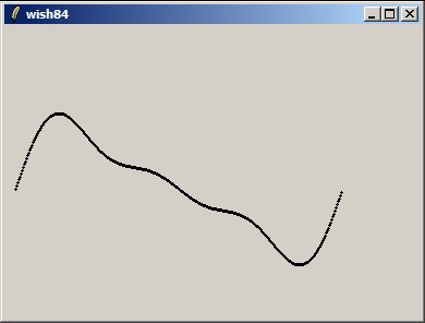
plotlist [additive {1.0 0.5  2.0 0.25  3.0 0.125} {300}] 

The resulting graph

The relevance of this, apart from that the above is a nice nested tcl function call, is that fourier synthesis as the reverse of fourier analysis is a powerfull tool in signal processing to make waveforms with known frequency spectrum with. If we take a number of sine waves added together, and preferably make an unsampled, infinite wave-function of them, then we have a perfectly frequency limited signal for all kinds of signal processing practices, like we could mathematically perfectly do in Maxima.

If we'd fourier transform these waves, they'd have perfect frequency spectrae, and especially also perfectly limited spectrea, which though filtering and other means is fundamentally impossible, then the theoretical spectrum is always without upper bound, which at some point in the computation can always lead to inaccuracies.

Even when making a tcl list of samples for these signals, this property of added sine waves, interpreted as one period of an infinite signal is very important: only these signals (and possibly some others created by appropriate methods, like the solution of differential equations) can be proven to comply with the Shannon Sampling Theorem, which allows us to take the tcl lists of samples as perfectly reconstructable samples, apart from the obvious vertical or amplitude discretisation: the numerical accuracy of the samples (for instance 13 digits or 32 bits floating point). So these are 'decent' sample lists.

And the power of this form of signal synthesis can be shown in tcl and our tk example as well: it can be shown that this sort of basis can span the whole real-valued function space, even orthonomally.

Important example are square and sawtooth waves, which we can approximate and show with the tk plot proc by chosing the right additive components, and which allow us to approximate such important waves (for instance in electronics or sound synthesis, but also when solving physics based differential equations) within any specified frequency range, so for instance exactly to fullfill a certain sample frequencies' shannon rate.

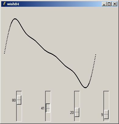
Maybe for demonstrations' sake it's a good idea to first make a set of sliders, with which we can interactively adjust an additively made spectrum, and accompanying wave.

# A frame to contain the sliders at the bottom
pack [frame .f] -side bottom -expand n -fill both

# wheneven one of the sliders is released, a new (corresponding) graph is made
proc updatefromsliders {} {
    global s1 s2 s3 s4
    set h [list 1.0 [expr {$s1/100.0}] 2.0 [expr {$s2/100.0}] 3.0 [
        expr {$s3/100.0}] 4.0 [expr {$s4/100.0}]]
    plotlist [additive $h 300]
}

# the scales (sliders)
scale .f.s1 -from 100 -to 0 -var s1
pack .f.s1 -side left -expand y -fill y
bind .f.s1 <ButtonRelease-1> { updatefromsliders }
scale .f.s2 -from 100 -to 0 -var s2
pack .f.s2 -side left -expand y -fill y
bind .f.s2 <ButtonRelease-1> { updatefromsliders }
scale .f.s3 -from 100 -to 0 -var s3
pack .f.s3 -side left -expand y -fill y
bind .f.s3 <ButtonRelease-1> { updatefromsliders }
scale .f.s4 -from 100 -to 0 -var s4
pack .f.s4 -side left -expand y -fill y
bind .f.s4 <ButtonRelease-1> { updatefromsliders }