Primal Screens
Primal Screens
or Investigating Prime Numbers when plotted in the Ulam Style — KWJ
Updated and corrected
Several years ago, this work was loosed on the wiki to describe a Prime Number Browser, which is a tool designed to answer some questions about the distribution of prime numbers when plotted in the Ulam Style. An excellent description and demonstration of the Ulam method by Gerard Sookahet, can be found on the Wiki at Ulam Spiral.
I've meant to rewrite this over the past several years, but have been interrupted many times. A strange side effect of the interruptions is that I've had to go back and figure out what had been done previously, and in the process, have discovered something new that I'd not seen before. Another reason for the delay is that discovery is way more fun than writing.
Browsers might be described as "aha!" generators, perhaps based on a conjecture by Yogi Berra who once said, "You can observe a lot just by watching". The Prime Number Browser displays prime numbers in the Ulam Style on two Primal Screens, one plotted as a Coarse Grid, the other as a Fine Grid. If we think of the integers from 1 to a very large number being connected like a string of pearls, then the Ulam method consists of laying them out in a spiral pattern on a square grid, with primes being blue pearls.
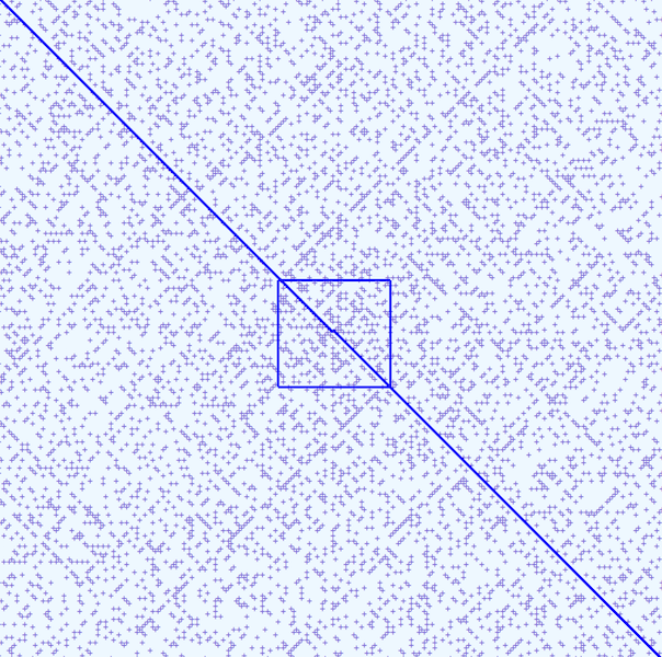
FIGURE 1
Figure 1 shows a portion of the set of prime numbers that are less than 100,000 (PLT100K), plotted on a Fine Grid. Instead of pearls, pluses represent prime numbers. As originally observed by Ulam, the primes do not fall in a random pattern, but certain directions are rich in primes.
On the plot are two blue diagonal lines which traverse the upper left and lower right quadrants. Although not obvious at this scale, these lines pass through integers which are perfect squares. The upper left line passes through numbers which are of the form y = m², where m is an even number. The lower right line passes through values where m is an odd number. Prime rich directions are either parallel or perpendicular to these lines. The blue lines are the Principle Axes in this representation.
In order to give a sense of scale, the blue square near the center represents the extent of the Coarse Grid, overlaid on the Fine Grid.
When carefully examined, Figure 1 reveals what looks like an empty channel running off from the center to the right. A similar vertical empty channel runs downward from the center toward the bottom of the grid. Several questions arise— "Are these channels truly empty? How far do they extend? Are there other directions which are depleted of Primes? Might there be some formulae that would generate such channels?" These were some questions the browser helped answer. Other obvious questions were — "Are there formulae that one might use to predict prime numbers along any of the prime rich directions? And what would those formulae look like?"

FIGURE 2
Figure 2 shows a smaller set of primes, plotted on the Coarse Grid. Here again, the blue lines are the Principle Axes. On this grid, the prime numbers are identified in blue and bold, non primes are in gray. The ability to see individual numbered cells in this manner was helpful in discovering possible Prime Predicting formulae and is the reason for the Coarse Grid.
Empty Channels
In Figure 2, the empty channels mentioned earlier appear as two rows of numbers extending off to the right, starting with the numbers 9 and 24. There are also two empty columns of numbers descending to the bottom, starting with numbers 20 and 22.
Regarding the question of whether formulae exist that predict empty channels, the Coarse Grid gives us a hint. The Principle Axes intersect numbers of the form, y = m², in which case, y is always non prime, thus an empty channel.
Just above the line of even squares we see what appears to be another empty channel containing numbers like 15, 35, 63, 99, etc. If the formula for the line of even squares, y = m² is modified by subtracting 1, we get the formula y = m² - 1. All numbers in this channel obey this formula. The equation can be rewritten as y = (m+1)(m-1), which is always non prime. A similar empty channel lies parallel and below the line of odd squares.
With these results, there is hope for finding formulae which predict prime numbers, based upon the lines of even and odd squares, the Principle Axes.
Prime Predicting Formulae
In figure 2, there is another line of prime numbers below the line of odd squares which run off to the bottom right, starting with the integers 7, 23, 47, 79, 167 etc. These primes are related to numbers on the line of odd squares in the following manner. 47 is two integers to the left of 49, which is 7², 79 is two integers to the left of 81, which is 9². Pursuing further, we see that these primes are all of the form y = m² - 2 for odd m.
Similarly there is a line of primes parallel to and beneath the line of even squares starting with the integers 43, 71, 107, 151, 263 etc. After searching around a bit, we find that 43 is seven greater than 36, which is 6². 71 is seven greater than 64 which is 8². The prime numbers along this line then, are of the form y = m² + 7 for even m. This is not to say that every number that the formula predicts are primes, but they do account for some primes along a certain prime rich direction. We will see later that there are other prime predicting formulae which are more potent at predicting primes than others.
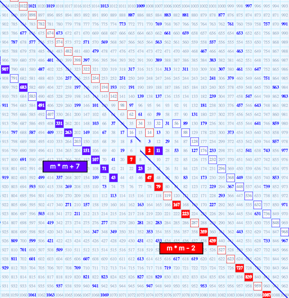
FIGURE 3
Figure 3 shows the results of the above two formulae plotted on the Coarse Grid. The set of primes of the form y = m² - 2 are displayed as Red squares, the non prime squares are White with Red outlines. For y = m² + 7 the primes are displayed as Blue squares and the non prime squares are White with Blue outlines.
Several things can be noted in this figure. First, each formula predicts a trajectory with two branches of numbers, one of which contains some primes, while the other branch appears empty of primes. Second, the branches empty of primes correlate with the sign of the second term in the formula y = m² + B. For B negative, non-primes are predicted for even values of m. For B positive, non-primes are predicted for odd values of m. There is a sort of confused region near the origin for small values of m, but at a certain point an asymptotic behavior develops into a line parallel to one of the principle axes. A question arises whether the asymptotic behavior continues for ever or might the trajectories bend further out.
Are There Other Kinds of Formulae?
About the time the above simple formulae were discovered, I stumbled on a very interesting reference at [L1 ].
This reference shows a table of polynomials which generate prime numbers. The emphasis of the table seems to be on polynomials which predict long continuous sequences of prime numbers. Many of the formulae there are more complex than the ones mentioned so far. I've limited my investigations to polynomials of second degree in m, and with smaller coefficients. Otherwise predictions soon exceed the prime number base of numbers that are less than 100,000.
It's interesting that those old rascals, Euler and Legendre had been down the path of Prime Number Generation a long time ago. Working diligently, probably by candle with quill and ink, Euler discovered the formula y = m² + m + 41 back in 1772. Some time later, Legendre proposed the formula y = m² + m + 17. Dropping these equations into the browser, we see something like Figure 4, plotted on the Coarse Grid.
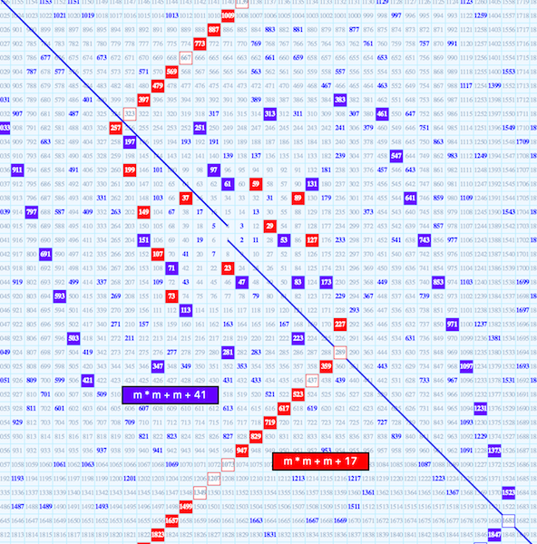
FIGURE 4
The Euler formula generates an impressive number of primes for the first 40 numbers for m = 0 to 39, but fails at m = 40. The Primes are plotted here on the Coarse Grid as Blue squares. The non primes are White squares with Blue outlines. Not quite as potent, but still impressive, the Legendre formula primes are plotted as Red squares and the non primes as White squares with Red outlines.
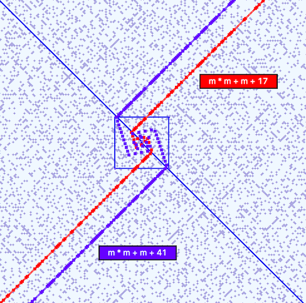
FIGURE 5
Figure 5 shows the trajectories of the above formulae when plotted on the Fine Grid. Note that both branches of these formulae contain primes. The primes for both trajectories are displayed as small colored squares, the non primes are small circles outlined in color (barely visible).
It's apparent that the Euler equation traverses one of the heaviest prime rich directions found in Figure 1. It also shows the characteristic "confused" region near the origin and then asymptotic behavior further out. Note also that the asymptotic direction for these formulae is perpendicular to that of the simpler equations of Figure 3.
Two More Interesting Formulae
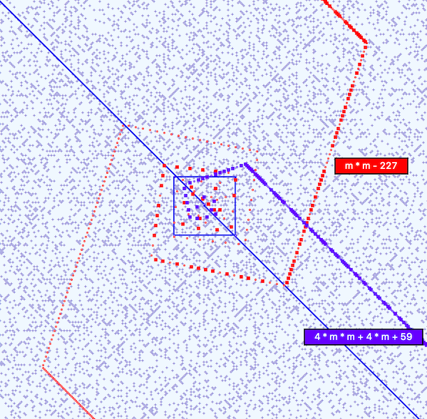
FIGURE 6
Figure 6 shows the trajectories of two more interesting formulae, and illustrates the value of a browser. The trajectory in Red was generated by y = m² - 227. Again, based on its simple polynomial form, we see two branches, one ultimately going to the left and downward, which is empty of primes, and the other going upward, containing primes. The second trajectory in Blue was generated by the formula y = 4m² + 4m + 59. In this case, both branches of the trajectory have collapsed into a single branch.
Both of these formulae illustrate the aha property of a browser. Until seeing this plot, my assumption was that a trajectory took on an asymptotic behavior that forever remained straight. It’s possible that trajectories really have bends if we look far enough out using larger sets of primes.
Potency
Another point of interest is what I call the Potency of a given prime predicting formula. This is the percent of Primes that an equation predicts out of the total number of predictions. The following table shows the potency for various formulae on the Coarse Grid and the Fine Grid:
| Potency | ||
|---|---|---|
| Formula | Coarse Grid | Fine Grid |
| M² - 2 | '0.238' | '0.211' |
| M² + 7 | '0.271' | '0.214' |
| Legendre | '0.457' | '0.457' |
| Euler | '0.803’ | '0.698' |
| M² - 227 | ‘0.350’ | ‘0.317’ |
| 4M² + 4M + 59 | ‘0.857’ | ‘0.641’ |
Whoops
While trying to finish writing this episode, I discovered that among the many formulae in 2 were the following two: y = m * m - 79 * m + 1601 and y = 2m² + 29. It turns out that the trajectory for the first formula almost exactly replicates Euler’s trajectory. However the browser says that it has a greater potency for the Fine grid, 259 Primes out of 354 Predictions for a Potency of 0.732.
Curious to see which new primes were predicted, a bit of sleuthing was done and it turns out that the formula duplicates some primes. In fact it produces 38 duplicates and ultimately predicts only one new prime— the number 41. Discounting the duplicates, the potency is 0.699 vs 0.698 for Euler’s formula. The following table shows some of these duplicates:
| m * m - 79 * m + 1601 | |
|---|---|
| m | Prime |
| 39 | 41 |
| 40 | 41 |
| 37 | 47 |
| 42 | 47 |
| 31 | 113 |
| 48 | 113 |
| 10 | 911 |
| 69 | 911 |
| 2 | 1447 |
| 77 | 1447 |
Currently one of many deficiencies of the browser is that it does not check for duplicate primes.
The formula y = 2m² + 29 mentioned above was also discovered by Legendre and has a greater potency than his previous formula, 0.640 vs 0.457. Plugging this into the browser, we get figure 7.
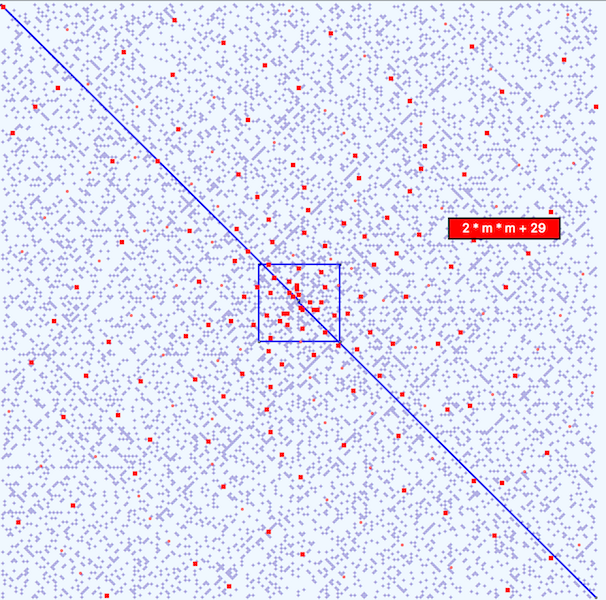
FIGURE 7
It turns out that the trajectory described by this formula is a spiral, quite unlike the previous straight line trajectories which go off in prime rich directions. How can that be? This will be explained in the next episode on Ulam Spirals Primal Screens— Part Two.
Something New
Until recently, my explorations had been confined to those prime numbers less than 100,000. Deciding to look further afield, I constructed a list of all primes less than 500,000 (PLT500K). There are 41538 of them, the largest being 499979. The result was a reaffirmation of Berra’s conjecture, ‘You can observe a lot by just watching’.
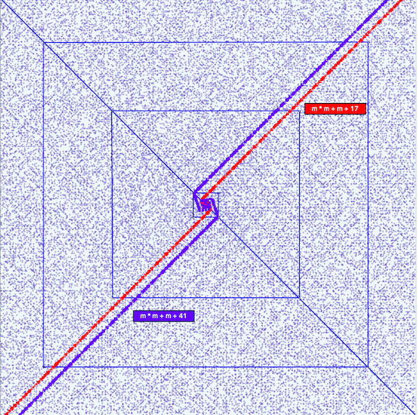
FIGURE 8
In this figure, the small blue plus marks (barely distinguishable at this resolution) represent the Prime Numbers. The first, inner Blue square is the limit of the Coarse grid, the next square represents prime numbers less than 100,000, the third square is the limit of all prime numbers less than 300,000 and beyond that are the rest of the primes less than 500,000.
With this set of primes, Euler’s formula is indeed remarkable, predicting 433 primes out of 706 predictions, for a potency of 0.613. Legendre’s formula predicts 278 primes out of 705 predictions- a potency of 0.394.
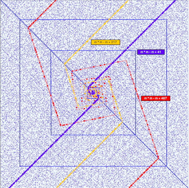
FIGURE 9
Figure 9 shows several other formulae which are in the spirit of Euler’s equation. The formula with 41 as the constant term is Euler’s. If we change the term to 217 and then 487, we see that bends occur in the trajectories further out as the constant term increases. These bends would not have been revealed had we limited ourselves to the PLT100K primes. Again, primes along these trajectories appear as the colored squares and the non primes are the small colored circles. In all three cases, primes exist on both branches.
Looking at this larger data set reveals another, unexpected, result. Some bends occur just as a branch crosses a Principle Axis and some of the straight segments are neither parallel nor perpendicular to the Principle Axes.
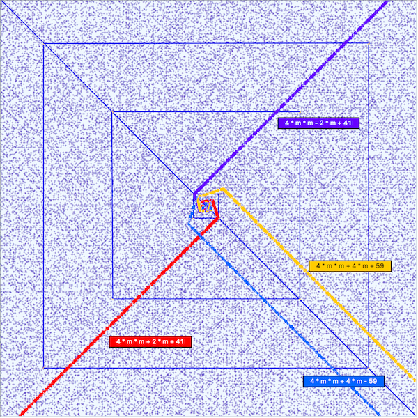
FIGURE 10
In Figure 10 we have trajectories for four different formulae. For each trajectory, both branches collapse into a single line. We saw the equation 4m² + 4m + 59 previously but only for the PLT100K set of primes. Here we see that the asymptotic behavior continues with no bends. The sign change in the 4m² + 4m - 59 formula illustrates how changing the sign of the constant term causes a mirroring effect in it’s trajectory. The two equations 4m² + 2m + 41 and 4m² - 2m + 41 show how the change in sign of the linear term effects the direction of the trajectories.
Tcl/Tk
This contribution is also meant to brag about Tcl/Tk, which was used to create the browser. Tcl’s flexibility and power have allowed me to easily pursue different questions as they came to mind. An example of such a question is figure 11, which is a plot of the set of Twin Primes that are less than 500,000. The question was, ‘Are there Twin-Prime Rich directions?’
From the following plot, it’s apparent that Twin-Prime Rich directions are not nearly as prominent as were the prime rich directions. Affixed to the plot, is Euler’s trajectory in red. It was fairly easy to address this question due to the power and flexibility of Tcl/Tk.
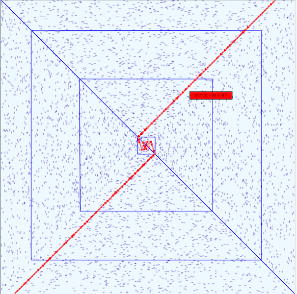
FIGURE 11
One Last Thing— Empty Channels Again
So, are there Formulae that predict the empty channels referred to in Figure 1 at the beginning? Yes, but at first, I wasn’t very excited about them. They just looked wrong, dividing by 2 seemed weird. But the following figure displays the horizontal and vertical channels that I first saw. It turns out that one of the branches of each trajectory is empty, while the other branch has a few primes. When first working with the various Formulae, I was not as tuned into this single empty branch behavior as I am now. These formulae will be important in the next episode Primal Screens— Part Two.
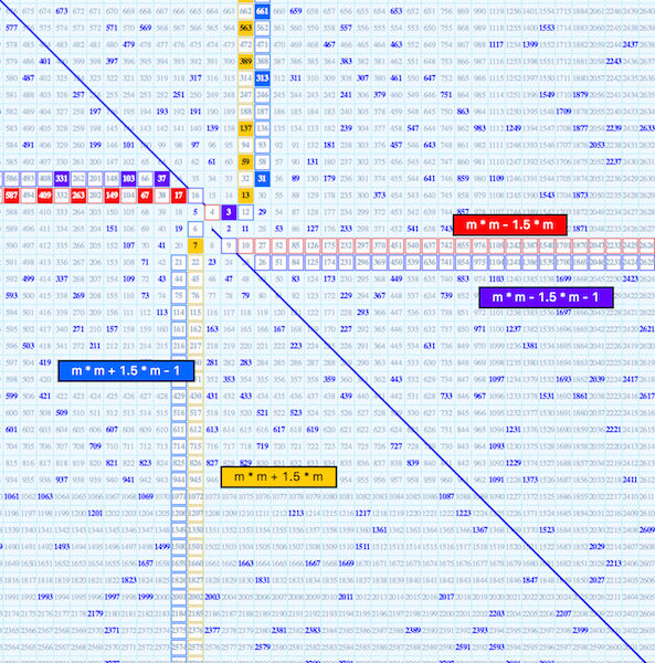
FIGURE 12
To conserve space, most all of the above plots have been reduced to 1/3 their normal size.
See also:
Primal Screens— Part Two and New Prime number Browser